Arithmetization

A proof system cannot directly reason about a program. Its algebra works with field elements, so the first step in any proof is to rewrite the statement as equations over a field. This rewriting is called arithmetization, and every later step depends on its output.

This chapter takes one small computation through the whole process. We start with ordinary arithmetic, express it as a list of multiplications and linear equations, and then compress all of those equations into a single equation with one secret vector. That final equation is the form Ragu proves, and the next chapter turns it into a statement about polynomials.

1. What arithmetization produces

We continue with the running example from the previous chapter:

I know a number $x$ such that $x^3+x+5=35$.

In the terms of that chapter, 35 is the instance and $x$ is the witness. Arithmetization has to produce a fixed set of equations, determined only by the statement's structure, such that a witness satisfies the equations exactly when the statement is true.

The equations cannot depend on the secret value, because the verifier must know them in advance. A program with an if branch therefore has to compute both branches and select one arithmetically. For example, a value $s$ is restricted to a bit by the equation $s(s-1)=0$, and the expression $s\cdot p+(1-s)\cdot q$ selects between $p$ and $q$. Hash functions and signature checks reduce to field equations in the same way, with many more of them.

All arithmetic in this chapter happens in ${\mathbb{F}}_{43}$, the scalar field of the toy curve from the curves appendix. The statement is an equation in this field, though the small values in our example make it look like ordinary arithmetic.

2. Flattening a computation

The expression $x^3+x+5$ contains several operations at once, so we first split it into steps that each perform one operation. Each intermediate result gets its own name:

The steps have different costs in a proof system. Step 3 is a linear combination of values we already have, and later sections show that linear combinations can be checked in bulk with a single random combination. Steps 1 and 2 multiply two unknown values, which no linear check can express. Multiplications are therefore what a proof system counts as its main cost, and we keep their number small.

3. Gates

Each multiplication becomes a gate. A circuit with $n$ gates uses three vectors $\mathbf{a},\mathbf{b},\mathbf{c}\in {\mathbb{F}}_q^n$, and gate $i$ requires

$$a_i\cdot b_i=c_i.$$

The entries of these vectors are called wires. Together they form the witness, which also goes by the name trace because it records one execution of the computation. In vector form, all the gates together say $\mathbf{a}\circ \mathbf{b}=\mathbf{c}$, where $\circ$ is the entrywise product.

Our computation has two multiplications, so $n=2$:

4. Linear constraints

The gates alone are not enough, because they treat every wire as independent. Nothing yet says that the $a_1$ of gate 1 is the output $c_0$ of gate 0, or that the same $x$ is used everywhere. A separate set of linear constraints connects the wires and ties them to the instance. Constraint $j$ has the form

$$\sum _{i=0}^{n-1}{u}_{j,i}{a}_i+\sum _{i=0}^{n-1}{v}_{j,i}{b}_i+\sum _{i=0}^{n-1}{w}_{j,i}{c}_i=k_j,$$

which we can write with inner products as

$$⟨{\mathbf{u}}_j,\mathbf{a}⟩+⟨{\mathbf{v}}_j,\mathbf{b}⟩+⟨{\mathbf{w}}_j,\mathbf{c}⟩=k_j.$$

The vectors ${\mathbf{u}}_j,{\mathbf{v}}_j,{\mathbf{w}}_j$ are public and describe the circuit. The vector $\mathbf{k}$ is the public input vector, which holds the instance.

Our statement needs four constraints. The first three connect wires, and the last one checks the output. It moves the constant 5 to the right side, which gives the target value $35-5$:

Step 3 from Section 2 has disappeared into constraint 3 at no additional cost in gates. This is why addition is cheap here: a sum of any number of wires appears as one row of coefficients, with no new multiplication.

Ragu allows up to $4n$ constraint rows, a limit that comes from the size of the polynomial holding the wiring data. Our circuit has room for 8 rows, and the four unused rows are all zeros, which any witness satisfies.

The gates and constraints together reject false statements:

Try $x=4$ instead. Filling in the gates gives $\mathbf{a}=(4,16)$, $\mathbf{b}=(4,4)$ and $\mathbf{c}=(16,21)$, with $4\cdot 4=16$ and $16\cdot 4=21$ modulo 43. Both gates and the first three constraints hold. The last constraint gives $c_1+a_0=25$, which is not 30, so this witness is rejected.

5. Reducing the gates to one equation

The verifier now faces $n$ gate equations and $4n$ constraints, and a real circuit has thousands of each. A proof that handled every equation separately would be enormous, so we want to replace them all with one equation that still fails if any of them fails.

Let $e_i=a_i{b}_i-c_i$ be the error of gate $i$. The previous chapter's random linear combination does this job, with the errors as the claims and the powers of a random value $z$ as the weights:

$$\sum _{i=0}^{n-1}{z}^i{e}_i=\sum _{i=0}^{n-1}{z}^i(a_i{b}_i-c_i).$$

This sum is a polynomial in $z$ with the errors as its coefficients, so it is 0 for every $z$ when all the gates hold. If any gate fails, the bound from that section applies, because the prover must fix the witness before seeing $z$. A uniformly random $z$ then hides the failure with probability below $n/|{\mathbb{F}}_q|$.

For the honest witness both gate errors are 0, so the sum is 0 for every $z$. Now take a dishonest witness with $\mathbf{a}=(3,8)$, $\mathbf{b}=(3,3)$ and $\mathbf{c}=(8,27)$. It satisfies all the linear constraints above, but its gate errors are $a_0{b}_0-c_0=1$ and $a_1{b}_1-c_1=40$ modulo 43. At $z=5$ the sum is $1+5\cdot 40=29$, which exposes the error. Checking all 43 values of $z$ finds 1 value that hides it, $z=29$, the root of this degree-1 polynomial.

On a field of about $2^{255}$ elements, this probability is negligible. We have traded certainty for an overwhelming probability, in exchange for checking only one equation.

6. Reducing the constraints to one equation

The constraints collapse in the same way, using a second random value $y$. Multiplying constraint $j$ by $y^j$ and adding gives

$$\sum _{j=0}^{4n-1}{y}^j(⟨{\mathbf{u}}_j,\mathbf{a}⟩+⟨{\mathbf{v}}_j,\mathbf{b}⟩+⟨{\mathbf{w}}_j,\mathbf{c}⟩)=\sum _{j=0}^{4n-1}{y}^j{k}_j.$$

Inner products are linear, so we can move the powers of $y$ inside. Define the combined vectors

$$\mathbf{u}(y)=\sum _j{y}^j{\mathbf{u}}_j,\mathbf{v}(y)=\sum _j{y}^j{\mathbf{v}}_j,\mathbf{w}(y)=\sum _j{y}^j{\mathbf{w}}_j.$$

The equation becomes

$$⟨\mathbf{u}(y),\mathbf{a}⟩+⟨\mathbf{v}(y),\mathbf{b}⟩+⟨\mathbf{w}(y),\mathbf{c}⟩=⟨\mathbf{k},{\mathbf{y}}^{4n}⟩,$$

where ${\mathbf{y}}^{4n}=(1,y,\dots ,y^{4n-1})$. The combined vectors are public once $y$ is known, so this is one linear equation in the witness.

At $y=7$, the combined vectors are $\mathbf{u}(y)=(37,7)$, $\mathbf{v}(y)=(42,6)$ and $\mathbf{w}(y)=(36,42)$. The left side for the honest witness is $2+15+39=13$ modulo 43. The right side is $7^3\cdot 30=13$, because only $k_3$ is nonzero.

We now have two equations, one quadratic in the witness and one linear. The remaining sections merge them into one equation about a single vector.

7. Reading one coefficient of a product

The merged equation needs a specific form, and the reason comes from polynomial multiplication. Take polynomials $p$ and $q$ with coefficient vectors $\mathbf{p},\mathbf{q}\in {\mathbb{F}}_q^m$. The coefficient of $X^k$ in the product $p(X)q(X)$ is the sum of $p_i{q}_j$ over all pairs with $i+j=k$. For the middle exponent $k=m-1$, this sum is

$$\sum _{i=0}^{m-1}{p}_i{q}_{m-1-i}.$$

Each entry of $\mathbf{p}$ meets the entry of $\mathbf{q}$ at the mirrored position. This is the inner product of $\mathbf{p}$ with the reversal $\hat{\mathbf{q}}$ of $\mathbf{q}$, which is called the revdot product:

$$⟨⟨\mathbf{p},\mathbf{q}⟩⟩=⟨\mathbf{p},\hat{\mathbf{q}}⟩=\sum _{i=0}^{m-1}{p}_i{q}_{m-1-i}.$$

Let $p(X)=1+2X+3X^2+4X^3$ and $q(X)=5+6X+7X^2+8X^3$ over ${\mathbb{F}}_{43}$. The coefficient of $X^3$ in $p(X)q(X)$ collects every pair of exponents that adds to 3: $1\cdot 8+2\cdot 7+3\cdot 6+4\cdot 5=17$ modulo 43. The revdot product computes the same sum, since $\hat{\mathbf{q}}=(8,7,6,5)$ and $⟨\mathbf{p},\hat{\mathbf{q}}⟩=17$. The full product has coefficients $(5,16,34,17,18,9,32)$, and the entry for $X^3$ is the one in the middle.

So a claim about a revdot product is a claim about one coefficient of a polynomial product. This link is why Ragu writes its checks as revdot products, and the next chapter uses it to reach a polynomial test. Our goal for the rest of this chapter is to express both equations as one revdot product.

8. Arranging the witness

A gate's product $a_i{b}_i$ has to appear in a revdot product of the witness with itself. Since revdot pairs position $k$ with position $m-1-k$, we need to place $a_i$ and $b_i$ at mirrored positions. We also need room for the $c_i$ wires, whose partners must not create unwanted products.

A vector of length $4n$ with four blocks of length $n$ achieves this:

$$\mathbf{r}=\mathbf{c}\Vert \hat{\mathbf{a}}\Vert \mathbf{b}\Vert \hat{\mathbf{d}}.$$

The vector $\mathbf{d}$ is an extra block of wires that we set to zero for now, so each $c_i$ has a partner of value 0. Reversing the $\mathbf{a}$ block places $a_i$ at position $2n-1-i$, and $b_i$ sits at position $2n+i$. These two positions add up to $4n-1$, so they are partners. A vector with this arrangement is called a structured vector.

With $n=2$, the positions and their partners are:

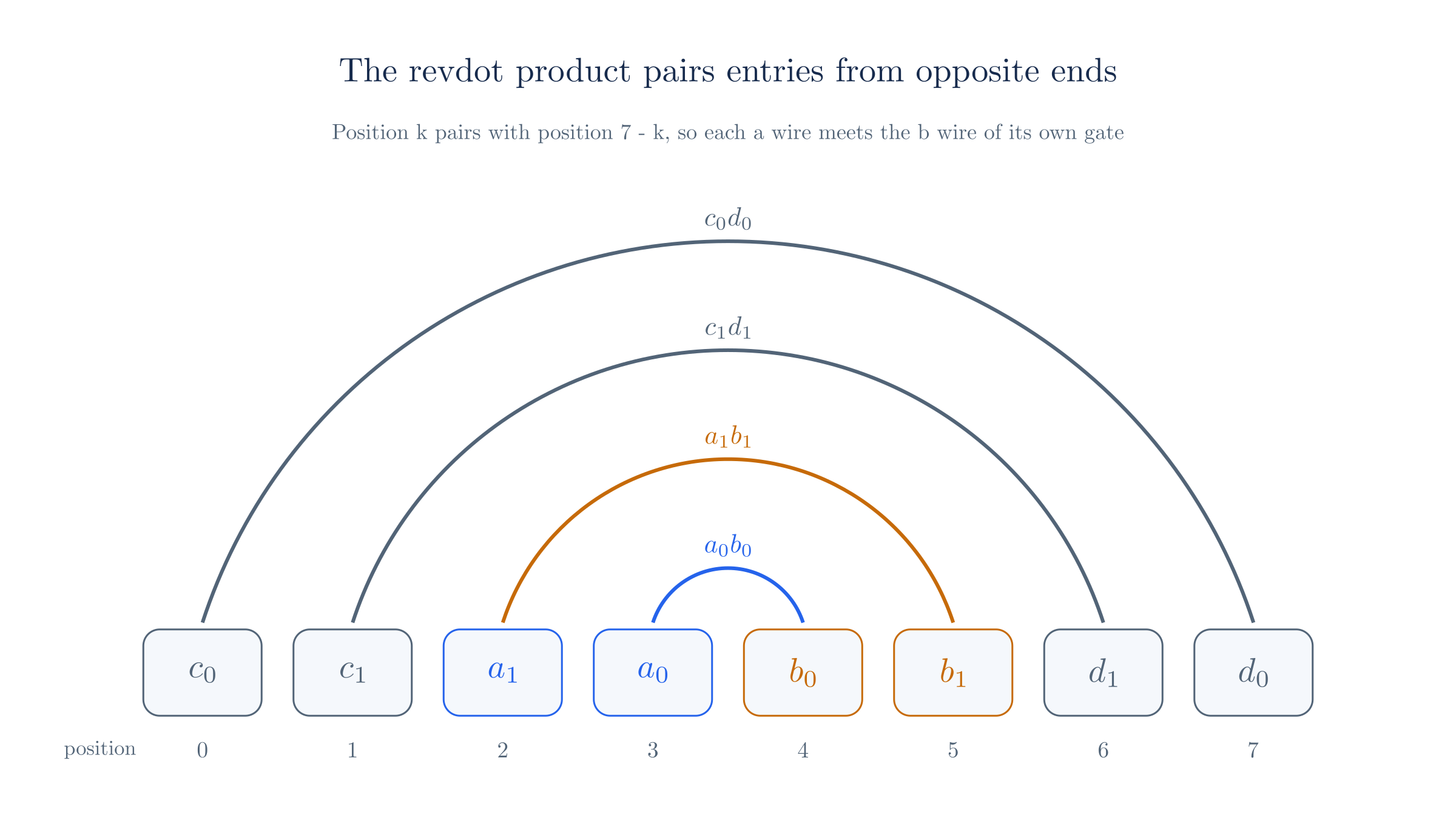
Each product appears twice in the revdot sum, once from each end of the pair. With $\mathbf{d}=0$, the $c$ wires contribute nothing, so

$$⟨⟨\mathbf{r},\mathbf{r}⟩⟩=2\sum _{i=0}^{n-1}{a}_i{b}_i.$$

For our witness, $\mathbf{r}=(9,27,9,3,3,3,0,0)$. Multiplying each entry by its partner and summing gives $⟨⟨\mathbf{r},\mathbf{r}⟩⟩=29$, and $2⟨\mathbf{a},\mathbf{b}⟩=2(3\cdot 3+9\cdot 3)=29$ modulo 43.

9. Weighting each gate

The sum $2{\sum }_i{a}_i{b}_i$ has lost track of which product belongs to which gate, so it cannot check the gates individually. Section 5 solved the same problem by giving each gate its own power of $z$, and we can build this weighting into the revdot product.

Multiply entry $k$ of the second vector by $z^k$. This operation is called dilation, and the result is $\mathbf{r}\circ {\mathbf{z}}^{4n}$, where ${\mathbf{z}}^{4n}=(1,z,\dots ,z^{4n-1})$. The revdot product becomes

$$⟨⟨\mathbf{r},\mathbf{r}\circ {\mathbf{z}}^{4n}⟩⟩=\sum _{k=0}^{4n-1}{r}_k{r}_{4n-1-k}{z}^{4n-1-k}.$$

Now we group the terms by gate. The wires $a_i$ and $b_i$ occupy positions $2n-1-i$ and $2n+i$. Taking $k=2n-1-i$ produces $a_i{b}_i{z}^{2n+i}$, and taking $k=2n+i$ produces $b_i{a}_i{z}^{2n-1-i}$. The pair of wires $c_i,d_i$ contributes in the same way at positions $i$ and $4n-1-i$. The result is

$$⟨⟨\mathbf{r},\mathbf{r}\circ {\mathbf{z}}^{4n}⟩⟩=\sum _{i=0}^{n-1}{a}_i{b}_i(z^{2n-1-i}+z^{2n+i})+\sum _{i=0}^{n-1}{c}_i{d}_i(z^i+z^{4n-1-i}).$$

Each gate now has its own weight, built from powers of $z$ that no other gate uses. With $\mathbf{d}=0$, the second sum vanishes.

At $z=5$ the powers are $(1,5,25,39,23,29,16,37)$, so $\mathbf{r}\circ {\mathbf{z}}^8=(9,6,10,31,26,1,0,0)$.

The last column sums to 38. The formula above gives the same value, using weights $z^3+z^4=19$ and $z^2+z^5=11$: $9\cdot 19+27\cdot 11=38$ modulo 43.

10. Removing the output wires

The expression above contains the products $a_i{b}_i$, but a gate check needs the differences $a_i{b}_i-c_i$. We therefore have to subtract $c_i$ with the same weight as its gate:

$$-\sum _{i=0}^{n-1}{c}_i(z^{2n-1-i}+z^{2n+i}).$$

This sum is linear in the witness, so it can be written as a revdot product of $\mathbf{r}$ with a public vector $\mathbf{t}$. The wire $c_i$ sits at position $i$, and its partner is position $4n-1-i$. Placing the desired coefficient at that partner position gives

$$t_{4n-1-i}=-(z^{2n-1-i}+z^{2n+i})\text{for }0\le i<n,$$

with all other entries of $\mathbf{t}$ equal to zero. Adding the two revdot products and using linearity gives

$$⟨⟨\mathbf{r},\mathbf{r}\circ {\mathbf{z}}^{4n}+\mathbf{t}⟩⟩=\sum _{i=0}^{n-1}(a_i{b}_i-c_i)(z^{2n-1-i}+z^{2n+i}).$$

This expression is the gate check from Section 5 with different weights. It is zero for every $z$ when all the gates hold, and otherwise it is a nonzero polynomial in $z$.

At $z=5$, $\mathbf{t}=(0,0,0,0,0,0,32,24)$. Its two nonzero entries sit at positions 7 and 6, the partners of $c_0$ and $c_1$. Then $⟨⟨\mathbf{r},\mathbf{t}⟩⟩=5$, and adding the dilated term gives $38+5=0$ modulo 43, as it should for a witness that satisfies its gates.

11. Encoding the constraints

The combined constraint equation from Section 6 is linear in the witness, so it fits the same pattern. We want a public vector $\mathbf{s}$ such that $⟨⟨\mathbf{r},\mathbf{s}⟩⟩$ equals its left side. Each wire's coefficient goes at the partner of that wire's position:

Filling in these entries gives $⟨⟨\mathbf{r},\mathbf{s}⟩⟩=⟨\mathbf{k},{\mathbf{y}}^{4n}⟩$ for a witness that satisfies the constraints.

At $y=7$, placing the vectors from Section 6 at the partner positions gives $\mathbf{s}=(0,0,6,42,37,7,42,36)$, and $⟨⟨\mathbf{r},\mathbf{s}⟩⟩=13$. This equals $⟨\mathbf{k},{\mathbf{y}}^8⟩=13$.

The vector $\mathbf{s}$ contains the whole circuit structure, compressed by $y$. The chapter on wiring and the registry studies how a verifier can check $\mathbf{s}$ without computing it from scratch.

12. The consolidated equation

Both checks are now revdot products with the same left vector $\mathbf{r}$. The revdot product is linear in its second argument, so we can add them into one equation:

$$\boxed{⟨⟨\mathbf{r},\mathbf{r}\circ {\mathbf{z}}^{4n}+\mathbf{t}+\mathbf{s}⟩⟩=⟨\mathbf{k},{\mathbf{y}}^{4n}⟩}$$

This is the output of arithmetization. It contains one secret vector, $\mathbf{r}$. Everything else depends only on the circuit, the instance, and the challenges $z$ and $y$.

At $z=5$ and $y=7$, the combined right vector is $\mathbf{r}\circ {\mathbf{z}}^8+\mathbf{t}+\mathbf{s}=(9,6,16,30,20,8,31,17)$. Its revdot product with $\mathbf{r}=(9,27,9,3,3,3,0,0)$ is 13, and $⟨\mathbf{k},{\mathbf{y}}^8⟩=13$. Checking the equation at all $43^2=1849$ pairs $(z,y)$ confirms that the honest witness passes at every pair.

Why a false witness fails

Subtracting the right side from the left side splits the equation into two parts:

$$\underset{E_g(z)}{\underbrace{\sum _{i=0}^{n-1}(a_i{b}_i-c_i)(z^{2n-1-i}+z^{2n+i})}}+\underset{E_c(y)}{\underbrace{(⟨⟨\mathbf{r},\mathbf{s}⟩⟩-⟨\mathbf{k},{\mathbf{y}}^{4n}⟩)}}=0.$$

The first part depends only on $z$, and every power of $z$ in it is at least $z^n$, since $2n-1-i\ge n$ for $i<n$. The second part depends only on $y$. A gate error therefore cannot cancel a constraint error for all values of the challenges, because the two parts vary independently. If either part is nonzero, the whole expression is a nonzero polynomial in $(z,y)$ of degree at most $4n-1$. The prover has to fix $\mathbf{r}$ before seeing the challenges, so a random pair passes with probability at most $(4n-1)/|{\mathbb{F}}_q|$. This bound is the two-variable Schwartz–Zippel lemma from the previous chapter.

On the toy field we can count the exact number of passing challenges for several dishonest witnesses:

The bound for this circuit is $(4n-1)/|{\mathbb{F}}_q|=7/43\approx 0.163$, and each row falls below it.

Those rates are large only because the field has 43 elements. For $n=2^{11}$ on a 255-bit field, the bound falls below $2^{-240}$.

Notice that the argument depends on the challenge order. A prover who learned $z$ and $y$ before fixing $\mathbf{r}$ could look for a witness that satisfies only this one equation. The chapter on polynomial commitments provides the tool that fixes $\mathbf{r}$ first.

13. The arithmetization in Ragu

14. Comparison with R1CS and PLONK

Other proof systems make different choices at this stage. Two of them are worth knowing, and the first is needed for the next chapter.

R1CS (rank-1 constraint system) uses one vector $\mathbf{w}$ containing the constant 1, the instance, and the witness. Three public matrices define the constraints:

$$A\mathbf{w}\circ B\mathbf{w}=C\mathbf{w}.$$

Each row is one constraint that multiplies two linear combinations of $\mathbf{w}$ and compares the result with a third. Our statement fits in three rows:

With $\mathbf{w}=(1,35,3,9,27)$, holding the constant 1, the public output, $x$, $w_1$ and $w_2$, the three matrices are

$$A=\left[\begin{array}{ccccc}0& 0& 1& 0& 0\\ 0& 0& 0& 1& 0\\ 5& 0& 1& 0& 1\end{array}\right],B=\left[\begin{array}{ccccc}0& 0& 1& 0& 0\\ 0& 0& 1& 0& 0\\ 1& 0& 0& 0& 0\end{array}\right],C=\left[\begin{array}{ccccc}0& 0& 0& 1& 0\\ 0& 0& 0& 0& 1\\ 0& 1& 0& 0& 0\end{array}\right].$$

The products are $A\mathbf{w}=(3,9,35)$ and $B\mathbf{w}=(3,3,1)$. Their entrywise product is $(9,27,35)$, which equals $C\mathbf{w}$.

R1CS and Ragu's system have the same expressive power, and each can be converted to the other with a linear increase in size. R1CS merges the wiring into its multiplication rows, while Ragu's system (called Bootle16, after its source paper) keeps gates and linear constraints apart. That separation is what makes the revdot form above possible.

PLONK uses gates with selectable coefficients, of the form $q_{L}a+q_{R}b+q_{O}c+q_{M}ab+q_C=0$, and adds separate copy constraints to connect wires. Later variants add custom gates and lookup tables that reduce the number of gates for certain operations. Ragu deliberately avoids these features. It uses a simple circuit model and splits large computations into many small circuits that communicate along the PCD tree.

15. Where this chapter leaves us

This chapter took the following steps:

1. A computation becomes a list of multiplication gates and linear constraints over a field.
2. Random powers of $z$ and $y$ reduce all gates and constraints to two equations, at the cost of a small failure probability.
3. A revdot product corresponds to one coefficient of a polynomial product.
4. A structured vector $\mathbf{r}$ places each $a_i$ and $b_i$ at mirrored positions, and dilation by $z$ weights each gate separately.
5. The public vectors $\mathbf{t}$ and $\mathbf{s}$ add the gate outputs and the wiring, which gives one equation.

The prover still has to convince the verifier of this equation without revealing $\mathbf{r}$. The next chapter starts from the R1CS form to derive the standard QAP reduction, and then uses Section 7 to reach a polynomial test for the consolidated equation.