Wiring and the Registry
Chapter 09 ended with two linear steps in the verifier. Accumulation dealt with the first, computing . This chapter deals with the second, computing , which requires reading the whole circuit. It also takes up a related problem that has waited since chapter 02, which is how different nodes of a PCD tree can run different circuits.
Both problems have the same answer. The prover commits to pieces of the wiring polynomial, a cheap random check ties each new piece to the old ones, and a single expensive check at the very end covers the whole history. The Ragu Book calls this idea post-processing, and credits it to Halo. We start with one circuit, then extend the method to a polynomial that holds many circuits, called the registry polynomial.
Reconstructed from code at commit 3219e08, not confirmed by the authors
The protocols come from the book's wiring consistency chapter and its registry chapter. The toy circuits, the attacks, and the link between a chosen circuit and its wiring value in Section 7 are our own assembly, and we read that link from the code. We could not read the Halo paper, so what we say about Halo follows the book. Section 13 compares everything with the code.
1. What the verifier still computes
Recall the check that ties the right factor to the trace in chapter 09,
The value has a short closed form, while the value has none, because the wiring comes from an arbitrary circuit:
Our circuit has 8 nonzero wiring coefficients, so computing takes 8 terms. A real circuit has at least one coefficient for each wire it uses, so at a full circuit needs on the order of 8,192 terms for this one value.
A recursive verifier would have to do this inside a circuit, so the circuit would have to contain a description of itself and grow with every wire it adds, as chapter 10 found. Chapter 11 escaped the same problem for by testing a claim at a random point, which worked because has a short product form. The wiring polynomial has no such form.
A natural next idea is to let the prover supply a commitment to and to carry the claim forward in the accumulator, as split accumulation does for evaluation claims. That chapter showed that folding establishes what opens to. It says nothing about whether commits to the right polynomial, and this gap is exploitable:
Take the false trace with , , at and . With the true wiring the revdot product is 18, and the target is . The prover adds to its wiring polynomial, which moves the revdot product by and reaches the target. It commits to the altered polynomial , which gives in place of the true . The right factor is built from this polynomial, so the check holds at all 43 values of , and every evaluation claim is true of the committed polynomials. The only thing wrong with this proof is that does not commit to .
So the claim has to be checked somehow, and we want the check to cost far less than computing . Polynomial identity tests are the usual tool for this, but a test needs a polynomial on the other side to compare with, and the verifier does not want to compute any of them. The next section finds that second polynomial inside itself.
2. Restricting a polynomial of two variables
The wiring polynomial has two variables. Its coefficients form a table, with one row for each constraint and one column for each position in the trace. Here is the table for our circuit, with empty cells for zeros:
| 42 | 1 | |||||||
| 1 | 42 | |||||||
| 1 | 42 | |||||||
| 1 | 1 |
We can fix either variable. Fixing gives a polynomial in , and fixing gives a polynomial in . Each of these is called a restriction. Both directions take the same table and add it up along different lines, so the two restrictions agree where they cross:
Fixing collapses the rows into , with coefficients . Fixing collapses the columns into , with coefficients on . These are different polynomials, and they meet at one number, since evaluating the first at and the second at both give .
This crossing is what the protocol uses. A commitment to a restriction in and a commitment to a restriction in make two evaluation claims that must have the same value, and chapter 08 already knows how to check evaluation claims cheaply. The verifier needs no knowledge of the table to compare the two claims.
Restricting in only makes sense if the result fits the commitment scheme, and this explains a limit we met earlier. The commitment has generators, so must have degree below in . The book gives this as the reason for the bound of constraint rows.
3. Consistency for one circuit
Suppose a node has two children, and each child's accumulator holds a claim of the form , meaning that commits to . The node wants to replace the two claims with one claim of the same form. We want three things from the replacement. It should tie each old to the true circuit, it should create a new claim at a fresh point, and it should leave no work that depends on the size of the circuit.
The book's protocol achieves this with a single restriction in that crosses all three restrictions in :
- Both parties hold the old claims and .
- The verifier sends a random .
- The prover sends , a commitment to .
- The verifier sends a random .
- The prover sends , a commitment to .
- Both parties add six evaluation claims to the batch of chapter 08.
Each pair of claims says that a restriction in and the restriction in agree at their crossing. The first two pairs concern the old claims, and the last concerns the new one:
Here we write for the value at of the polynomial behind a commitment , as the book does. We now run this on our circuit, using two accumulators with values we have already met. The first holds chapter 09's , and the second holds the of chapter 12's second proof:
| Step | Party | Value |
|---|---|---|
| 1 | Both hold | and |
| 2 | Verifier sends | |
| 3 | Prover sends | , the commitment to |
| 4 | Verifier sends | |
| 5 | Prover sends | , the commitment to |
The prover states one value for each pair, which gives six claims about four polynomials:
| Claim | Commitment | Point | Value | Which value is shared |
|---|---|---|---|---|
| 0 | 21 | 35 | ||
| 1 | 7 | 35 | ||
| 2 | 21 | 6 | ||
| 3 | 34 | 6 | ||
| 4 | 21 | 2 | ||
| 5 | 12 | 2 |
The verifier never computes these values. It treats them as claims that share polynomials and places them in the batch, so one number in each pair appears twice:
With , and , the prover sends and the values at , one for each of the four polynomials: . The verifier derives , then and . A decider holding commits to it and evaluates it, and both results match. Checking the crossing identity at all 1849 pairs confirms that an honest prover passes at every challenge.
A batched check tells us that the claims are true of the committed polynomials, and it says nothing about the circuit. Something still has to connect the last commitment to the real wiring. That job falls to the end of the chain, in the same way that a single MSM ended chapter 11's chain:
The accumulator that leaves this fold is . If the chain stops here, the decider computes from the circuit, which takes 8 terms, commits to it and gets . That one linear computation stands in for computing at each of the three points.
4. Why a false accumulator fails
The argument runs backward from the decider. Suppose the decider has confirmed that commits to . Then the third pair of claims fixes to the correct value, and the prover committed to before it saw . Two different polynomials of degree below agree at no more than points, so is , except with probability about . That makes correct, so the first pair fixes to the correct value, and the prover fixed before it saw . The same reasoning then shows that commits to .
We can follow this in the toy run by giving the prover a false and counting what it can do at each step. Say it holds an built for the attack of Section 1. The first check it faces is the pair at :
The most favourable false polynomial differs from by a multiple of , the difference that chapter 09 found best for its cheater. Against an honest , the pair of claims about can hold only where this difference vanishes. Trying all 43 values of finds 7 that pass, . No polynomial with 8 coefficients has more roots.
Outside those values the prover must lie in to keep the pair true, which moves the error one step along:
At the false opens to , while the true is . The prover can absorb this error by committing to with and , so that both old pairs now hold. The polynomial can have at most 7 roots, and one of them has to be . Taking the other six at , we tried all 43 values of against an honest , and 7 pass.
Outside those values the error moves once more:
At the difference is , so the prover has one option left. It commits to , which opens at to the value that now requires. All six claims are true of the committed polynomials, and the batched check of the previous section accepts. The prover has moved its error into the new accumulator, whose commitment is . The decider computes itself, gets , and rejects.
So a false accumulator does not disappear. At each step it either hits a rare root or it passes its error into a new commitment, and the decider exposes the last one. A chain that never runs the decider has established nothing about its wiring, in the same way as chapter 12's evaluation claims.
All of this depends on the order of the messages. If the prover knows before fixing , then the pair at tests nothing:
Suppose the prover knows before it fixes the old accumulator. The difference , scaled by , vanishes at that point and gives the revdot shift of Section 1, so the false polynomial passes with an honest and an honest , and the decider accepts the accumulator that leaves the fold.
This is why the old commitments have to enter the transcript before is squeezed.
5. A polynomial for many circuits
The protocol above assumes that every accumulator refers to the same . Now suppose a tree has two kinds of step. We will use the running circuit as circuit A, along with a second circuit B that has the same number of gates and proves a different statement:
| Circuit | Statement | Constraints that differ from A | Commitment | |
|---|---|---|---|---|
| A | None | |||
| B | and |
The two accumulators may now refer to different circuits, and the bridge of Section 3 stops working, since a single cannot be a restriction of both:
Let the first accumulator hold circuit A at and the second hold circuit B at , so that . If commits to , the first pair of claims holds, and the second compares with . Over all 43 values of these agree only at , so an honest prover with two different circuits fails almost everywhere.
We could avoid this by merging A and B into one large circuit with a selector, as chapter 04 did for a branch. Then every step would pay for the gates of all its branches, which is the cost chapter 02 wanted to avoid. A better way is to keep the circuits apart and to put the choice of circuit into the polynomial itself, as one more variable.
Pick a set of points , one for each circuit, where is a root of unity of order . Let be the Lagrange polynomial that equals 1 at and 0 at the other points, as in chapter 05. The registry polynomial is
Setting makes every term vanish except one, so . The field needs enough roots of unity for this. The toy field has nonzero elements, so its only roots of unity of 2-power order are and , and our registry holds exactly two circuits. With two points, the Lagrange polynomials are and :
| 1 | 0 | , which is | |
| 0 | 1 | , which is | |
| 29 | 15 | , which is neither |
The script compares with and with at all 1849 pairs, and they agree at every pair. Since at every , the two weights at also add up to 1, and we return to this fact in Section 10.
The last row of that table shows what does away from the domain. It gives a blend of the circuits that belongs to no single one, and the protocol uses this blend as a random fingerprint of the whole set.
An accumulator now has to carry a claim that does not name one circuit, so that accumulators from different circuits can merge. The form the book chooses leaves free. The claim is , meaning that commits to , the polynomial in that holds every circuit's value at the point . Section 7 shows why this form is also the one we want for reading a single circuit's value. Since this polynomial is committed with the same generators, it needs degree below in , and the code enforces that a registry has at most entries.
6. Consistency for the registry
Two old claims and now differ in two coordinates, while the claims in Section 3 differed in only one. A single bridge cannot cross both, so we change one variable at a time. The book's protocol freezes at a random point, moves to a common value, moves to a common value, and then lets go free again. Here are its steps:
- Both parties hold the old claims.
- The verifier sends a random .
- The prover sends and , commitments to and .
- The verifier sends a random .
- The prover sends , a commitment to .
- The verifier sends a random .
- The prover sends , a commitment to .
- Both parties add ten evaluation claims to the batch.
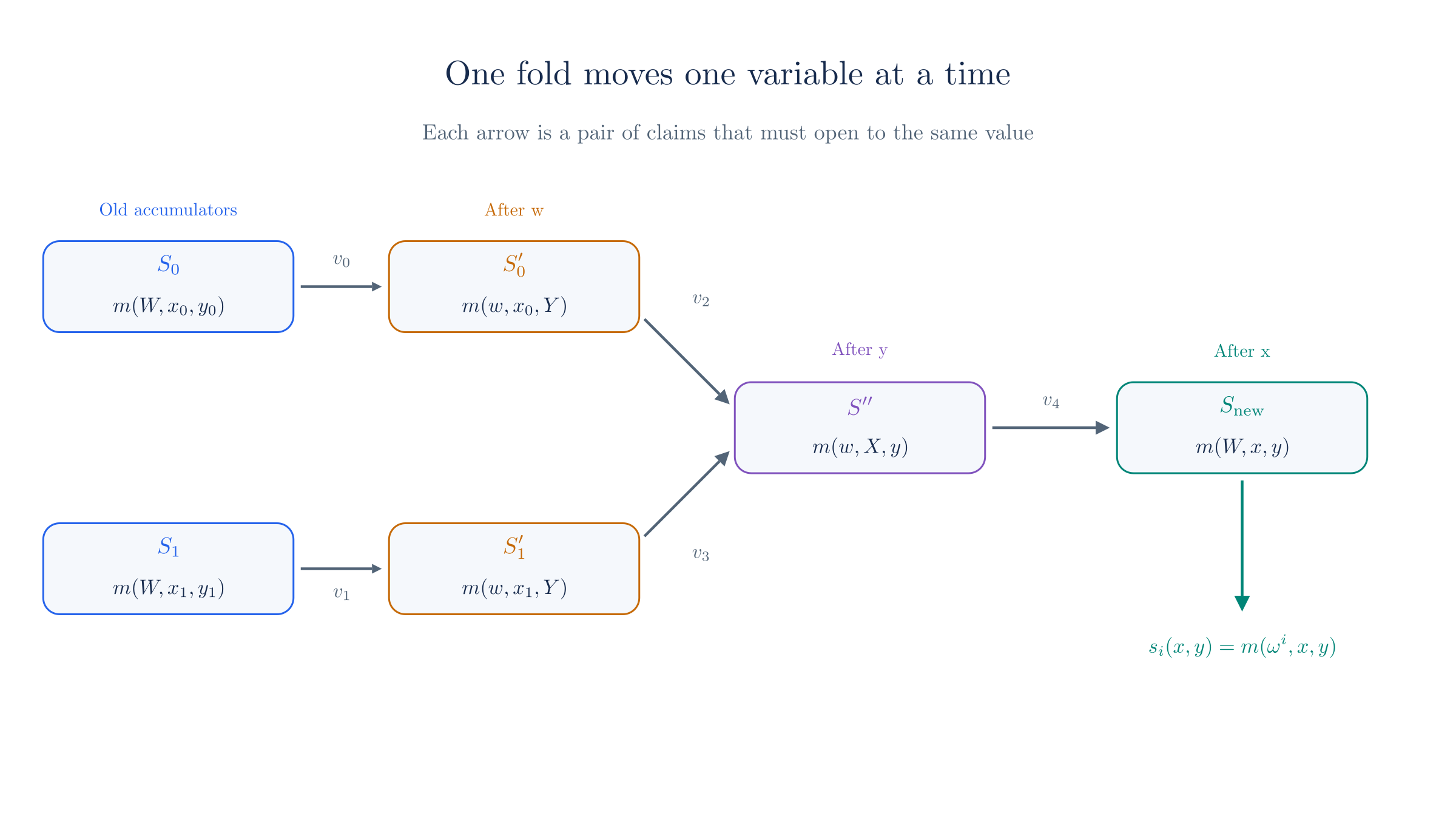
Each arrow in the figure stands for a crossing of two restrictions, and each crossing gives a pair of claims:
Two bridges are needed in step 3 because the children have different . Only one is needed in step 5, because at that point both children have the same , and both restrictions in land on the same polynomial in .
For the toy run, let the left child have used circuit A at chapter 09's challenges, and the right child circuit B at the and of chapter 12's second proof:
| Step | Party | Value |
|---|---|---|
| 1 | Both hold | and |
| 2 | Verifier sends | |
| 3 | Prover sends | for |
| Prover sends | for | |
| 4 | Verifier sends | |
| 5 | Prover sends | for |
| 6 | Verifier sends | |
| 7 | Prover sends | for |
Notice that the commitment to uses only the first two generators, because on this domain it has degree 1 in . The five crossings give the following values:
| Shared value | Number | First claim | Second claim |
|---|---|---|---|
| 10 | at 14 | at 7 | |
| 7 | at 14 | at 34 | |
| 42 | at 12 | at 9 | |
| 26 | at 12 | at 37 | |
| 12 | at 21 | at 14 |
The script repeats these comparisons at all 79,507 triples , and an honest prover passes every one.
The accumulator that leaves the fold is , and it has the same form as the two that entered, so the next node can repeat the walk.
7. Selecting a circuit
The walk keeps the accumulators consistent with , but the point of all this was to obtain the value for the check in Section 1, for whichever circuit a child used. The new accumulator provides that value directly. Since commits to , opening it at the domain point of circuit gives
This is why the accumulator leaves free. Each circuit's value is one evaluation claim on the same commitment, and the prover names the circuit by naming the point. The check from Section 1 then reads a claimed value that the batch will test, in place of a value the circuit would have to compute.
The new accumulator is . Take , so that . For each child the circuit reads the wiring value by opening at the child's domain point, and it adds the trace value and the gate value:
| Child | Sum, | ||||
|---|---|---|---|---|---|
| Left, circuit A | 2 | 21 | 23 | 3 | |
| Right, circuit B | 17 | 7 | 23 | 4 |
The script also confirms that each child's revdot product at and equals its own , with different wiring and different public inputs on the two sides.
The two children here used different wiring and the same step of the protocol handled both. Only the evaluation point changed. These two openings bring the list to twelve claims, on six polynomials:
With , and , the prover sends and six values at : . The verifier derives , then and , and a decider holding accepts. The wiring decider then evaluates the accumulator at a fresh point. At the polynomial gives , and the two circuits give .
The last sentence of that run is the registry's form of the decider, and we describe its cost next.
8. What the registry costs
The cost divides among three parties. The recursive circuit handles claims only, whatever the size of the registry or of the circuits. It does a little field arithmetic per claim, as in chapter 12, and the six commitments join that chapter's list. It also checks that each child's circuit point lies in the domain, which takes squarings per child, as Section 10 explains. Here is a comparison for a hypothetical tree with 256 application circuits of gates each, which is the gate limit chapter 10 recorded:
| Approach | What one step puts in its circuit | Size for this example |
|---|---|---|
| Compute directly | One term per wiring coefficient of each child's circuit | At least 16,384 multiplications for two full circuits |
| One merged circuit with selectors | The gates of every circuit, on every step | 524,288 gates |
| Registry, as in this chapter | Field arithmetic on claims, 6 commitments in the fold, and a domain check on 2 indices | 12 claims and 16 squarings |
The prover pays more than this table suggests. Each of the four new polynomials is a Lagrange-weighted sum over the circuits, so computing one touches every registered circuit, including those the step did not use. The book describes a floor planner and memoization that let circuits with common routines share this work, which is one source of the "diminishing overhead" it claims. We have not measured these costs.
The decider pays too. To test it computes at a fresh , which means one for each circuit. That is a linear cost in the total size of the registry, and the compressed verifier evaluates at several points of the walk, but all of this happens once for a whole history.
Adding a circuit therefore leaves the recursive circuit almost unchanged, so the book encourages applications to split work into many small circuits that communicate along the PCD tree, and it speaks of hundreds or thousands of circuits. Tachyon, which has not activated on mainnet and whose design is still changing, has a few dozen steps at the revision we read, and those steps run against a mock of Ragu.
9. Assigning domain points
The formula in Section 5 gives circuit the point , but depends on , and depends on how many circuits there are. If a registry grows from four circuits to five, it moves from a domain of 4 points to one of 8, and then changes and so does the point of every circuit except the first. Circuit code that refers to another circuit's point would then need to know the final count. The toy field has no room to show this, so we use in this section, for arithmetic only. Its multiplicative group has order , so it has a root of unity of order . Write for the element of order , with .
| Circuit | Naive, 4 points: | Naive, 8 points: | Bit-reversed, any size |
|---|---|---|---|
| 0 | 1 | 1 | 1 |
| 1 | 22 | 64 | 96 |
| 2 | 96 | 22 | 22 |
| 3 | 75 | 50 | 75 |
The first two columns differ at every circuit except the first, and the 8-point column gives circuit 2 the value that the 4-point column gave circuit 1. To avoid this, we take one maximal domain, of order where is the largest power of 2 dividing the group order, and assign each circuit a point there. Circuit gets , where is with its bits reversed. The book calls this rolling domain extension, and the third column above uses it.
Reversing the bits puts the low bits of at the top of the exponent, so small values of give exponents that are multiples of a large power of 2:
| Circuit | in 5 bits | Reversed | Exponent | Order | |
|---|---|---|---|---|---|
| 0 | 00000 | 00000 | 0 | 1 | 1 |
| 1 | 00001 | 10000 | 16 | 96 | 2 |
| 2 | 00010 | 01000 | 8 | 22 | 4 |
| 3 | 00011 | 11000 | 24 | 75 | 4 |
| 4 | 00100 | 00100 | 4 | 64 | 8 |
| 5 | 00101 | 10100 | 20 | 33 | 8 |
| 6 | 00110 | 01100 | 12 | 50 | 8 |
| 7 | 00111 | 11100 | 28 | 47 | 8 |
The last column shows why this works. The first circuits always land on elements of order at most , which are exactly the -th roots of unity. They fill the small domain first, and growing the registry adds new points without moving old ones. The element also stays the same when written in the smaller domain, since for , which the script checks at every size. So a circuit can compute its own point, or another circuit's, from its index alone. The code's omega_j does this, and a test asserts the orders 1, 2, 4, 4, 8, 8, 8, 8 that the table shows.
On the largest available 2-power order is 2, so . Circuit 0 gets , and circuit 1 gets , which are the two points our registry has used all along.
The degree of in still depends on , because the Lagrange polynomials change with the domain. What stays fixed is the element that names each circuit.
10. What the prover may select
The prover chooses the point at which opens for each child, and a verifier should worry about a free choice like this. We go through the three things the prover might choose.
A point outside the domain
The fact from Section 5 that the Lagrange weights add up to 1 now causes trouble. A point outside the domain gives a blend of circuits with , and that blend behaves as a third circuit that nobody registered. We need the constant wire of chapter 09 to show this, so this section uses circuits of 3 gates, with and :
Take the instance , whose second coefficient is the public output, and let the prover select the out-of-domain point . There the weights are and , and they add up to 1, so and the mixture looks like a circuit. The input does not satisfy , yet the trace with , which is , satisfies the consolidated equation at all 1849 pairs . The same trace passes against circuit A at 43 pairs and against circuit B at 43. The domain check catches the selection, because , which is not 1.
So the protocol has to check the point. A value is in the domain exactly when squaring it times gives 1, and the hashes_1 circuit enforces this on both children's points. The uncompressed and compressed verifiers make the same check on the root's point.
A domain point with no circuit
The domain usually has more points than circuits, because is the next power of two. The registry also holds bonding polynomials, which chapter 17 uses for its stage checks, and which enforce the relation on a partial trace. A prover might select one of these in place of a circuit.
The book treats every domain point as a wiring polynomial. An unassigned point holds the zero polynomial, and it counts as a bonding polynomial. The two kinds differ in one coefficient. A circuit has the constraint at , so , while a bonding polynomial leaves that constraint out, so . Here is a registry with three entries on a domain of 4 points in :
| Circuit index | Domain point in | What sits there | |
|---|---|---|---|
| 0 | 1 | , a circuit | 1 |
| 1 | 96 | , a circuit | 1 |
| 2 | 22 | A bonding polynomial | 0 |
| 3 | 75 | Nothing registered, so the zero polynomial | 0 |
The verifier always sets when it expects a circuit, and this rules out the second kind. To see this, read the consolidated equation at , as a statement about the coefficient of . A bonding polynomial contributes nothing to that coefficient, so the only terms left on the left side are the gate terms from chapter 04,
and these would have to equal 1 for every . Only the term with in the second sum contains , and it brings with it, so a constant 1 cannot be formed.
Take the trace with and the instance , and let the prover select the zero polynomial. Its gates hold, so the left side is 0, and the equation becomes , which holds for one value of . Over all 1849 pairs it passes at 43. A prover can try to manufacture the missing 1 from the terms by setting , with an instance that has no public outputs. Then the left side is , because the term at always comes with a partner at . It equals 1 only at , which is 43 of the 1849 pairs.
A different registered circuit
The two checks above leave the prover a free choice among registered circuits. That choice is safe only if the statement says which circuit it expects, and a public input with the same shape can otherwise be proved by the wrong circuit:
Suppose the verifier wants a proof that some satisfies . Trying all 43 values shows that no such exists, so this statement is false. The verifier computes , and the prover selects circuit A in place of circuit B, with . Every check passes at all 1849 pairs, because the instance is the same as that of the true statement . Now add a row to each circuit that sets the linear coefficient of to a value fixed for that circuit, 2 for A and 3 for B, and let the verifier compute . Circuit B with a true output, such as and the output 40, still passes everywhere. The same substitution with circuit A now passes at 43 of the 1849 pairs, all of them at .
The extra row plays the part of the header suffix from chapter 02. The book's substitution section says that an application circuit's suffix fills the linear coefficient of , and that application suffixes are nonzero. Internal circuits output suffix zero, so they cannot pass as application circuits. The code applies this to every internal circuit slot. In the code a suffix belongs to a header type and not to one circuit, so unlike our toy row it leaves steps with the same output header interchangeable.
11. Post-processing and the registry tag
We can now say what is unusual about this design. Many recursive systems preprocess each circuit into a verification key, a short commitment to the circuit's polynomials, and the verifier reads this key. With many circuits, a recursive verifier would have to handle a table of keys. Ragu has no such keys, as its book states. A verifier holds the registries themselves, built from the circuit definitions, and a prover computes the restrictions it needs at each step. That is the sense in which the work moves from before the proof to after it.
Without keys, one question remains, which is how the transcript comes to depend on the circuits. Fiat–Shamir requires the statement to enter the transcript before any challenge, and the circuits are part of the statement. Here is what goes wrong otherwise:
Fix the false trace and suppose the transcript has produced and from data that does not depend on the circuit. At these values the trace misses its target, because constraint 3 is off by . An author who has seen can now publish a slightly different circuit, whose constraint 0 reads . This constraint fails on the trace by , and with its weight that exactly cancels the error of constraint 3 with its weight . Two constraints are broken, and the equation holds at . Counting over all 1849 pairs, it holds at 129, namely those with , so the verifier was misled only because the circuit came after the challenge.
The usual fix is to hash the circuits into the first transcript state. That does not work directly here, for a reason the code documents. The registry contains the recursive verifier's own circuits, and those circuits replay the transcript, so a transcript that starts from a digest of the registry would need that digest inside the circuits that it summarizes. Keyed systems avoid the cycle because they generate the key beforehand and carry it in public inputs.
Ragu breaks the cycle with a registry tag, a field element added to the polynomial at the one slot that no circuit uses:
We should first check that this cannot break an honest proof. Read as a constraint, the term is at row , and at its partner in the revdot product is position 0 of the trace, the wire . So it adds the constraint , which holds for every , because the system gate has . The code reserves that row by refusing a circuit that would reach it. The term has no factor of , so it appears at every domain point, and it vanishes at , so it does not disturb the distinction of Section 10.
Take . On the trace of chapter 09's constant-wire circuit, , the wire is 0, and the tagged wiring polynomial still satisfies the consolidated equation at all 1849 pairs. The tag cannot be added to our earlier two-gate circuit, whose . There the term contributes , and the honest trace passes at only 43 pairs, those with . The tag reaches every commitment a fold makes to a restriction. For the commitment to is , and going through all 43 values of gives 43 different points. So a transcript that absorbs this commitment gives challenges that the author of the circuit could not predict before was drawn.
The order of events is what provides the protection. The whole system description, including every circuit, is fixed and published first, and then is sampled independently and without bias. An author cannot adapt a circuit to challenges that depend on a number drawn after the circuit was published. The code keeps one tag for each of its two registries.
A temporary mechanism
The book and the code both call the caller-supplied tag a temporary workaround for issue #78, which replaced an earlier tag derived from evaluations. Each application has to supply its tags, for example from a public randomness beacon, and the API does not verify how they were produced. Any argument that needs a nonzero tag has to include the small chance that uniform sampling returned zero. Expect this part of the design to change.
12. Why cheating fails
This argument is informal. It assumes the discrete log relation assumption for the generators, it treats the transcript hash as a random oracle with each challenge drawn after the data it tests, and it assumes that someone runs the decider. It also assumes that the circuit ties each child's and circuit point to that child's proof, for the reason that chapter 12 gave about dropping an accumulator. A prover who could restate and freely could prove consistency for coordinates that have nothing to do with the check they were meant to support.
The reasoning of Section 4 applies to the registry link by link. Each commitment is tested at a challenge drawn after it was fixed, and a false commitment passes only at a root of its difference from the true polynomial. Running the toy registry with the best difference we could build at each link gives these counts:
| False commitment | Variable left free | Challenge that tests it | Passing values out of 43, with the best difference |
|---|---|---|---|
| 7 | |||
| 7 | |||
| 7 | |||
| The next , or the decider's | 7 |
The right child's commitments behave in the same way as the left child's. Those rates are large because the field is small and the polynomials have 8 coefficients:
At on a field of about elements, each link passes with probability at most . Adding this over the six commitments of one fold gives , which is below .
Now take the attack that opened this chapter and try it against the full protocol. The prover no longer gets to supply a free , because its wiring value has to come out of the accumulator at the domain point of the circuit it named:
Replay Section 1 at and . The false trace needs a wiring value of at , while the true is . That value comes from at , so the prover has to change this polynomial, and it can do so without disturbing the claim at or the right child's value by adding . All twelve claims are true of the committed polynomials, and the batched check accepts. The false accumulator commits to in place of . The next check tests it at a fresh point. Over all 43 values, the only ones that pass are and , the two points the prover built into its difference.
That false accumulator then behaves as in Section 4. It moves from node to node, it changes form with each fold, and at the end of the chain the decider rejects it. As chapter 12 showed, this conclusion relies on binding, because a prover who knows a relation among the generators could open the same point to a different polynomial.
13. Wiring and the registry in Ragu
The code at commit 3219e08 runs the walk of Section 6 inside fuse on both of its registries. Its test-oracle verifier states what each stage must hold, and this list locates most of the values from our table in Section 6 and the two openings from Section 7. Here m is the registry polynomial, left_id is the left child's domain point, and the first entry is the value shared by and :
let query_claim = claimed
    == [
        m(w, x, y),
        m(w, left_x, left_y),
        m(left_id, x, y),
        m(w, left_x, y),
        m(w, right_x, right_y),
        m(right_id, x, y),
        m(w, right_x, y),
    ];
The book and the code use different names for the same objects:
| This chapter | Polynomial | Book | Code |
|---|---|---|---|
A child's registry_xy | |||
registry_wx0, registry_wx1 | |||
registry_wy | |||
registry_xy | |||
| The registry tag | Tag, and in its comments | ||
| A circuit's point | CircuitIndex::omega_j, and in comments |
We use because already names the public input polynomial.
Reconstructed from code at commit 3219e08, not confirmed by the authors
- Message order. The fuse squeezes after the preamble, which carries the children's stored commitments, and then commits to the two . It squeezes and together, commits to , and later squeezes and commits to . The order matches Section 6, with the revdot messages of chapter 14 in between.
- The claims. The static query list names all ten claims of Section 6, then the two openings at the children's circuit points, and the
compute_vcircuit gives each claim its value. - Internal circuits. The fuse also opens at each internal circuit's fixed point, so the real list has more entries than our twelve. Those values feed the check of for internal circuits in the same way as an application circuit's value.
- The order of registration.
finalizeplaces internal circuits first, then bonding polynomials, internal steps and application steps, which gives the internal circuits low indices. - The decider. The test-oracle verifier samples a fresh and compares the stored polynomial with , computed from the registry. In production, compression turns this into an opening of the commitment at , whose value the verifier computes from the registry. That is the final linear cost that chapter 18 places in the larger picture.
- Two registries. The nested registry runs the same walk at the nested counterparts of the challenges, on the other curve of chapter 13's cycle. Its query list has no openings at children's circuit points, which agrees with that chapter's finding that application circuits sit only on the native side.
The Ragu Book and the code differ here
The S commitment. The book's wiring chapter opens with a commitment to for the circuit at hand, and its NARK and its claim list include such an . We found no such per-circuit commitment in the fuse. The code adds into and reads from , as Section 7 describes.
The list of claims. The book's registry protocol lists ten claims and stops, so it does not say how a chosen circuit's value reaches the check of . The code adds the openings at circuit points. This site follows the code.
Domain points. The book's wiring chapter writes and notes that this ignores the remapping. The opening of its registry chapter says that circuits go to successive powers of , while its later section and the code use bit reversal. Sections 5 to 7 use as the book's simplification does, and on the toy domain the two agree.
Memoization. The book's routines chapter describes a memoized evaluation path, and a code comment calls a multi-dimensional strategy planned under issue #58. We did not establish how much of this applies to the registry at this commit.
14. Where this chapter leaves us
This chapter took the following steps:
- Without a check against the circuit, a prover can commit to wiring of its own and satisfy every other part of the proof.
- Two restrictions of a polynomial agree at their crossing, which turns a claim about wiring into a pair of evaluation claims.
- For one circuit, a restriction ties old claims to a new claim, and a false claim either hits a rare root or passes its error forward until a decider rejects it.
- The registry polynomial holds many circuits, each at a root of unity, and its restriction lets a single commitment supply any circuit's wiring value.
- The registry walk moves , and one at a time, using four new commitments and ten claims, and each child's circuit adds one more claim.
- The recursive circuit pays a fixed cost for any registry size, while the prover and the decider pay for reading all of the circuits.
- Bit reversal gives each circuit a point that does not depend on the size of the registry.
- A domain check rules out blended circuits, rules out bonding polynomials and unassigned points, and a header suffix tells apart circuits whose output headers differ in type.
- No verification keys exist, so the transcript depends on the circuits through a registry tag that is sampled after they are published, and the code treats this tag as a temporary measure.
This completes the three linear subprotocols that chapter 09 listed: evaluation claims in chapter 12, revdot products in chapter 14, and wiring here. All of them produce challenges in one field and use them on commitments handled in another, so the next chapter looks at how a challenge can cross the curve cycle cheaply.