Curve Cycles

The recursive proofs chapter set a problem aside. A circuit that verifies a proof has to add and scale commitments, and the coordinates of those commitments live in a different field from the circuit's wires. The accumulation chapter ignored the same problem, and the split accumulation chapter worked on one curve as if it did not exist. This chapter deals with it.

We first measure what it costs to compute in the wrong field, and the cost turns out to rule that route out. We then introduce a second curve whose coordinates match the first curve's scalars, divide each fold between two circuits so that each one does only native arithmetic, and handle the two problems this division creates. The two circuits have to see the same data, and they have to use the same challenges. The chapters on staging and endoscalars later give the full mechanisms for these two problems, so here we only explain why each is needed and show the idea on the toy cycle.

1. Two fields in one commitment

Here is the fold from chapter 08, which a recursive step has to check:

$$\begin{array}{rl}P& ={\beta }^m\cdot F+\sum _{i=0}^{m-1}{\beta }^{m-1-i}\cdot C_i,\\ v& ={\beta }^{m}f(u)+\sum _{i=0}^{m-1}{\beta }^{m-1-i}{p}_i(u).\end{array}$$

These two lines look alike, but they ask for different arithmetic. The polynomials have coefficients in ${\mathbb{F}}_{43}$, the scalar field of the toy curve $E$. The second line is therefore a computation in ${\mathbb{F}}_{43}$, and a circuit over ${\mathbb{F}}_{43}$ can do it with one gate per multiplication. A circuit has to be over this field because its own trace is a polynomial that gets committed on $E$, and commitments on $E$ take scalars in ${\mathbb{F}}_{43}$.

The first line adds and scales points of $E$, and the addition formula from the recursive proofs chapter works on coordinates, which lie in ${\mathbb{F}}_{31}$. We can see what happens if we run that formula on the wrong wires:

Take the commitments $(27,30)$ and $(6,23)$ from chapter 08. Modulo 31 the slope is $21$ and the sum is $(5,29)$, a point on $E$. Run the same three formulas on wires that reduce modulo 43 and the slope becomes $29$, and the result is $(34,25)$, which lies on neither curve of the toy cycle.

The formula fails because each of its multiplications needs a remainder modulo 31, and the wires produce a remainder modulo 43:

The first gate of that addition checks $\lambda \cdot (x_2-x_1)=y_2-y_1$, which here reads $21\cdot 10=24$ modulo 31. As integers, $21\cdot 10=210$, and $210$ leaves remainder $24$ modulo 31. A wire in ${\mathbb{F}}_{43}$ holds $38$, because that is the remainder modulo 43, and the remainder modulo 43 says nothing about the remainder modulo 31.

So a circuit over ${\mathbb{F}}_{43}$ handles the value $v$ directly but has no direct way to handle the point $P$. On real curves the same mismatch holds, and the two fields have no useful relation between their remainders.

2. Emulating the other field

A circuit can still check a multiplication modulo 31 if it treats the numbers as integers. The prover supplies a remainder $r$ and a multiple $t$, and the circuit checks the integer equation

$$a\cdot b=r+31t.$$

If this holds over the integers and $r$ is small, then $r$ is the product modulo 31. The difficulty is that a gate can only check equations modulo 43, and the two sides of this equation are often larger than 43, so a false witness can match:

The honest witness for $210$ is $r=24$ and $t=6$, since $24+31\cdot 6=210$. A single gate can only check this equation modulo 43. Of the $992$ pairs with $r$ below 31 and $t$ below 32, $23$ satisfy it, and $22$ of those have the wrong remainder. One of them is $r=0$ and $t=4$, because $0+31\cdot 4=124$, which equals $210$ modulo 43.

The way out is to make every equation the circuit checks so small that it cannot wrap around modulo 43, because an equation between small numbers modulo 43 is also an equation between integers. We split $a$, $b$, $r$ and $t$ into pieces called limbs. On the toy field each limb is one bit, so $a={\sum }_i{a}_i{2}^i$ with five bits, and similarly for the others. We also write $31t=32t-t$, which keeps the terms small. Expanding $ab-r-32t+t$ and collecting by powers of 2 gives one column per power:

$$ab-r-31t=\sum _k(\sum _{i+j=k}{a}_i{b}_j-r_k+t_k-t_{k-5})2^k.$$

This sum has to be zero, but each column does not have to be zero, since a column can carry into the next one as in ordinary addition. So the circuit takes a witness carry $c_k$ for each column and checks

$$\sum _{i+j=k}{a}_i{b}_j-r_k+t_k-t_{k-5}+c_{k-1}=2c_k,$$

with $c_{-1}=0$ and the last carry equal to 0. Here is the first gate of our addition, written in columns:

Here $a=21$ and $b=10$. Each row satisfies its equation and the last carry is 0. The gates are $25$ for the products $a_i{b}_j$, $10$ to show that the bits of $r$ and $t$ are bits, and $18$ for the $9$ carries at $2$ bits each, since an honest carry always lies between $0$ and $3$. That is $53$ gates for one multiplication in ${\mathbb{F}}_{31}$. We ran the check on all $31^2$ pairs $(a,b)$ against all $32^2$ pairs $(r,t)$. It accepted $961$ inputs, one for each pair $(a,b)$, and each of them had the true remainder.

One native multiplication has become dozens of gates. The cost multiplies through every point operation, since the formulas are built from these multiplications:

A 6-bit scalar multiplication on $E$ does 5 doublings and 5 additions, or $35$ multiplications in ${\mathbb{F}}_{31}$ at $53$ gates each. With its selections and scalar bits, it costs $1,911$ gates, where the same operation on $E^{\prime }$ costs $51$ gates in the recursive proofs chapter. That leaves out the extra work to reduce the sums and differences in each formula back into range.

A real field has room for larger limbs, which lowers the count per bit. The next estimate is our own plain design and not a gadget that Ragu contains, and better gadgets exist that cut these numbers by some factor:

Take the same plain design with 4 limbs of 64 bits. One multiplication then uses $16$ limb products, $510$ bits for $r$ and $t$, and $7$ carries of about $67$ bits, for about $995$ gates. A point addition needs three of these, or about $2,985$ gates, which already exceeds the $2,048$ gates that Ragu allows in one circuit. A 255-bit scalar multiplication needs $1,778$ multiplications, or about $1,769,110$ gates, where the native version costs $2,541$. Apart from the MSM for $\hat{G}$, the verifier of Chapter 09 has $32$ such multiplications, which comes to about $56,611,520$ gates.

The book calls non-native arithmetic prohibitively expensive, and these counts show why. The accumulator's whole purpose was to keep the verifier small, and this one requirement would undo it. We need a way to avoid computing in the wrong field at all.

3. A curve for each field

The recursive proofs chapter already used the way out, when it counted gates on the partner curve $E^{\prime }$, since the coordinates of that curve lie in ${\mathbb{F}}_{43}$:

Take the points $(34,3)$ and $(40,18)$ on $E^{\prime }$. Their slope and sum are computed modulo 43, so every gate works in the circuit's own field. The addition takes $3$ gates and gives $(29,31)$, which we confirmed lies on $E^{\prime }$.

It may look as if we could move everything to $E^{\prime }$, but $E^{\prime }$ has 31 points, so its scalars lie in ${\mathbb{F}}_{31}$. A commitment on $E^{\prime }$ holds a vector over ${\mathbb{F}}_{31}$, and it cannot hold the polynomials of a circuit over ${\mathbb{F}}_{43}$. Those polynomials need $E$, and the points of $E$ need wires in ${\mathbb{F}}_{31}$. A circuit over ${\mathbb{F}}_{31}$ would then have its own polynomials, which $E^{\prime }$ can commit to, and those points need wires in ${\mathbb{F}}_{43}$. The two curves fit together in this way because of how their numbers of points were chosen:

We call this a 2-cycle of curves. It is a pair of prime fields ${\mathbb{F}}_p$ and ${\mathbb{F}}_q$, with a curve over ${\mathbb{F}}_p$ that has $q$ points and a curve over ${\mathbb{F}}_q$ that has $p$ points. Each circuit can do the point arithmetic for the polynomials of the other. Ben-Sasson, Chiesa, Tromer and Virza introduced the use of such cycles for recursive proofs.

A single curve whose number of points equals the size of its field would avoid the need for a partner, but such a curve is called anomalous, and discrete log on anomalous curves is easy by a known attack due to Smart, Semaev, and Satoh and Araki. So two curves are the smallest arrangement that works.

The Hasse bound says that a curve over ${\mathbb{F}}_p$ has $p+1-t$ points with $|t|\le 2\sqrt{p}$, which means the two primes of a cycle must be close together:

For $E$ we have $31+1-43=-11$, and $2\sqrt{31}$ is about $11.1$. For $E^{\prime }$ we have $43+1-31=13$, and $2\sqrt{43}$ is about $13.1$. Both differences fit within the bound.

Pairs of curves with this property are uncommon, even among small primes:

We counted the points on every curve $y^2=x^3+b$ over each of the $21$ primes below 200 that are congruent to 1 modulo 3. Among the $210$ pairs of these primes, $10$ form a cycle, and the pair $(31,43)$ is one of them. The same count finds $5$ primes with a curve whose number of points equals its field size, starting with $7$.

4. The Pasta cycle

Ragu uses the Pasta curves, which Chapter 01 explained are already deployed in Orchard and in hardware wallets. Pallas is the curve $y^2=x^3+5$ over ${\mathbb{F}}_p$ with $q$ points, and Vesta is the curve $y^2=x^3+5$ over ${\mathbb{F}}_q$ with $p$ points, where

$$\begin{array}{rl}p& =\text{0x40000000000000000000000000000000224698fc094cf91b992d30ed00000001},\\ q& =\text{0x40000000000000000000000000000000224698fc0994a8dd8c46eb2100000001}.\end{array}$$

Both are primes of 255 bits, and $q-p$ has only 87 bits, which is below the size that $2\sqrt{p}$ allows. We tested the cycle property directly. A point found on $y^2=x^3+5$ over ${\mathbb{F}}_p$ goes to the identity when multiplied by $q$, a point over ${\mathbb{F}}_q$ goes to the identity when multiplied by $p$, and only one multiple of each prime lies within the Hasse range, so the two orders must be $q$ and $p$.

The next table lines up the names we will use. The field of the main circuit is ${\mathbb{F}}_p$, and the code commits that circuit's polynomials on Vesta, whose scalars are ${\mathbb{F}}_p$ and whose coordinates are ${\mathbb{F}}_q$. The toy cycle plays the same roles, with one difference in size. In the toy cycle the main circuit has the larger field, while in Pasta it has the smaller one, and this does not affect the construction.

The two fields are close in size, but their elements are not interchangeable, because a value can be in range for one and out of range for the other:

In the toy cycle, $12$ of the 43 values of ${\mathbb{F}}_{43}$ are 31 or larger, so more than a quarter of them have no equal in ${\mathbb{F}}_{31}$. In the Pasta cycle the fraction is near $2^{-167}$, so a random value of ${\mathbb{F}}_q$ almost always fits in ${\mathbb{F}}_p$. A protocol still cannot rely on that for values a prover can choose.

Section 9 returns to this when challenges have to cross between the circuits.

5. Recursion on a cycle

With two curves there are two kinds of circuit, and every recursive step now uses both. The book calls this a ping-pong pattern. There is a primary circuit $C{S}^{(1)}$ over ${\mathbb{F}}_p$ and a secondary circuit $C{S}^{(2)}$ over ${\mathbb{F}}_q$. Each has its own polynomials, committed on its own curve, so each has its own accumulator. Where the split accumulation chapter had one ${\mathsf{acc}}_i$, we now have a pair $({\mathsf{acc}}_i^{(1)},{\mathsf{acc}}_i^{(2)})$.

Each accumulator contains both field elements and points, and the rule for dividing the work follows from Section 1. Field elements are native to the circuit that made the polynomial, and points are native to the other circuit. The book states the split for the whole accumulator, including the $\bar{A}$, $\bar{B}$ and $c$ that the revdot folding chapter introduces. For the batched claim $(P,u,v)$ it gives:

So the update of each accumulator is split between the two circuits, and each circuit updates half of each accumulator.

Timing matters as well. A circuit's commitments do not exist until its trace is complete, so a step cannot fold its own trace. The book's rule is that the instances produced in step $i$ are folded only in step $i+1$. The trace of the primary circuit in step $i$ becomes a commitment on $E$, whose coordinates the secondary circuit can read, so the secondary circuit folds that point in step $i+1$. The same holds in the other direction:

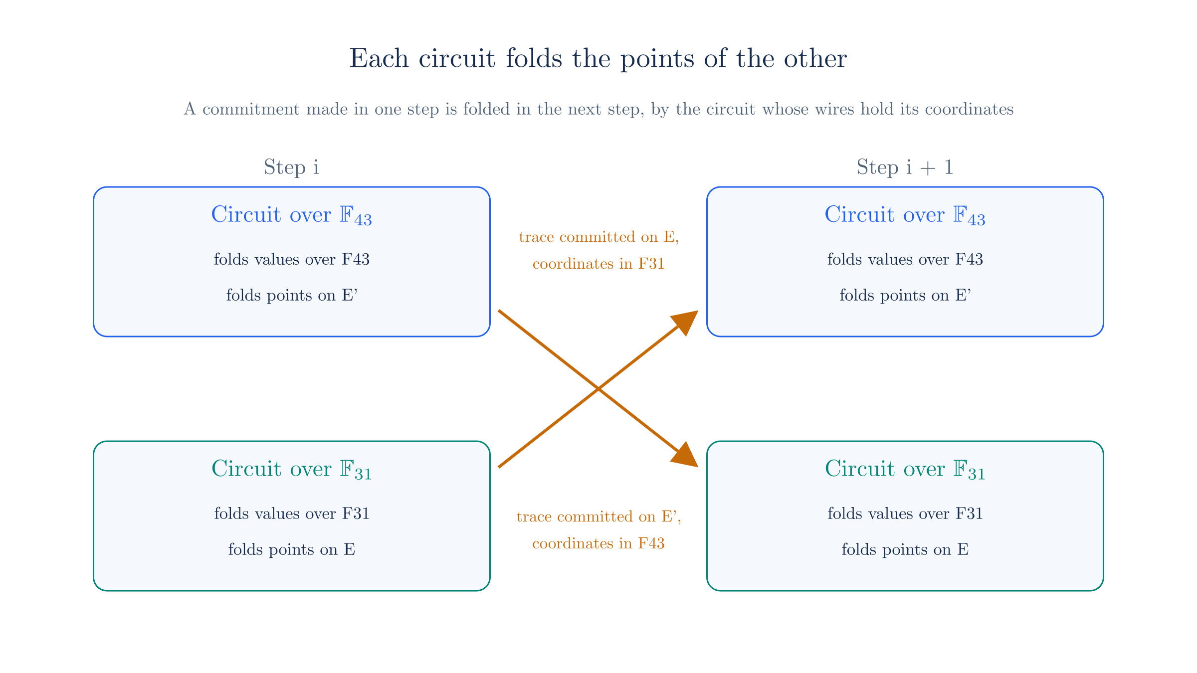
Everything from the recursive proofs chapter about trees carries over. A node holds two children, each with a pair of accumulators, and it folds both into one new pair.

6. A fold split across two circuits

Here is one fold on the toy cycle. We take two claims on each curve. The first side reuses chapter 08's polynomials, and the second side uses two new polynomials over ${\mathbb{F}}_{31}$ committed with four generators of $E^{\prime }$.

The prover runs chapter 08's batching on each side, with the same three challenges on both:

The challenges are $\alpha =11$, $u=13$ and $\beta =15$, each picked by hand and each below 16, for a reason that Section 9 gives. On the first side, the prover's quotient combination is $f=(20,36,37,0)$ with commitment $F=(28,10)$, and the values at $u$ are $30$ and $8$. On the second side, it is $f^{\prime }=(6,2,9,0)$ with commitment $F^{\prime }=(13,21)$, and the values at $u$ are $1$ and $1$.

Now we assign each output to the circuit where it is native. For a value, the circuit inverts each $u-x_i$, multiplies by the difference $p_i(u)-y_i$, and accumulates with powers of $\alpha$ and then of $\beta$. For a point, it runs the Horner form of the first equation in Section 1, starting from the commitment to $f$ and using the plain double-and-add from the recursive proofs chapter on the 4-bit $\beta$:

The prover also holds the combined polynomials $p=(7,4,23,6)$ and $p^{\prime }=(23,30,16,2)$. A decider commits to them and gets $(17,24)$ on $E$ and $(20,40)$ on $E^{\prime }$. Evaluating at $u=13$ gives $14$ in ${\mathbb{F}}_{43}$ and $9$ in ${\mathbb{F}}_{31}$. All four numbers match the table.

The saving is what this arrangement is for:

The tracer that runs these gates refuses any point whose coordinates are not in its own field, and every run above passed that test. The point $P$ took $68$ gates on wires in ${\mathbb{F}}_{31}$. If the circuit over ${\mathbb{F}}_{43}$ had computed it by the method of Section 2, the same steps would have cost at least $2,612$ gates.

The table hides two assumptions. The secondary circuit computed $P$ from the commitments on $E$ and the primary circuit computed $v$ from claims about those same polynomials, but nothing yet connects what the two circuits read. A prover could give each a different set of inputs. The two circuits also used the same $\alpha$, $u$ and $\beta$ only because we typed the same numbers. The book names these problems input consistency and challenge consistency. The next three sections address them.

7. Committing to coordinates

The primary circuit derives challenges by hashing the transcript, as the recursive proofs chapter required, and the transcript has to contain the commitments that the challenges test. For a commitment on $E$, this means absorbing coordinates from ${\mathbb{F}}_{31}$ into a sponge over ${\mathbb{F}}_{43}$. A circuit cannot do that natively, and the book also rules out hashing all the inputs on both sides and comparing the digests, since that needs either non-native arithmetic or bit decompositions of every value.

The cycle gives a neater route. The coordinates of a point on $E$ are elements of ${\mathbb{F}}_{31}$, and ${\mathbb{F}}_{31}$ is exactly the scalar field of $E^{\prime }$. So we can place the coordinates in a vector and make an ordinary Pedersen commitment to it on $E^{\prime }$. The result is one point on $E^{\prime }$, whose coordinates lie in ${\mathbb{F}}_{43}$. The book calls this a nested commitment, and it writes $\mathring{A}$ for the nested commitment to data involving $A$:

Take $A=(27,30)$ and $B=(6,23)$. Their coordinates form the vector $(27,30,6,23)$ in ${\mathbb{F}}_{31}^4$. Each entry is a valid scalar on $E^{\prime }$, so we commit with four generators of $E^{\prime }$, namely $(32,3),(34,3),(35,21),(37,7)$:

$$\mathring{A}=27\cdot G_0^{\prime }+30\cdot G_1^{\prime }+6\cdot G_2^{\prime }+23\cdot G_3^{\prime }=(12,12).$$

The coordinates of $\mathring{A}$ lie in ${\mathbb{F}}_{43}$, so the circuit over ${\mathbb{F}}_{43}$ can hold them as wires and absorb them. The toy sponge over ${\mathbb{F}}_{43}$ takes those two values and squeezes the output $2$.

In this way, one small point can stand for any number of foreign points. The commitment binds them under the same assumption as any Pedersen commitment, now for the generators of the second curve:

Changing the first coordinate to each of the other $30$ values gives $30$ different points, and $28$ of those change the sponge's output as well. A vector of four entries from ${\mathbb{F}}_{31}$ has $923,521$ possible values and $E^{\prime }$ has only 31 points, so collisions must exist. Here is one found by solving a discrete log: since $G_0^{\prime }+26\cdot G_1^{\prime }=\mathcal{O}$, the vector $(28,25,6,23)$ gives the same point.

Both circuits need to read all of the step's data, which includes four kinds of values. The primary circuit is native to values in ${\mathbb{F}}_{43}$ and to points on $E^{\prime }$, and the secondary circuit is native to values in ${\mathbb{F}}_{31}$ and to points on $E$. The book's encoding for the primary circuit handles them in two layers. The values and points that it can read go directly into a part of its own trace, which gives a commitment $C$ on $E$. Then $C$, the points of $E$ and the values in ${\mathbb{F}}_{31}$ all form one vector over ${\mathbb{F}}_{31}$, and the nested commitment to this vector is a point with coordinates in ${\mathbb{F}}_{43}$. The secondary circuit's encoding mirrors this, so that each circuit holds what it can read as wires and holds the rest behind one commitment.

The prover computes a nested commitment outside the circuit and supplies it as a witness. So at this stage the primary circuit knows that it hashed some point, and it does not yet know that the point contains the coordinates that the secondary circuit used. The next section adds that connection.

8. Deferred operations

Suppose the primary circuit's fold needs $s\cdot A$ for some point $A$ on $E$. It holds only $\mathring{A}$, so it cannot compute this. The nested commitment binds the data without carrying over any operation on it. The secondary circuit has the coordinates of $A$ as wires and can do the multiplication, so the work moves there, and we call it a deferred operation.

For this to mean anything, the wires that the secondary circuit uses have to be the same values that $\mathring{A}$ commits to. The tool for this is a staged trace, which the staging chapter covers in full. The prover splits the secondary circuit's trace into two polynomials,

$$r(X)=A(X)+r^{\prime }(X),$$

where $A(X)$ holds the coordinates in slots reserved for it and $r^{\prime }(X)$ holds everything else. It commits to each part separately, and the commitment to $A(X)$ is the nested commitment that the transcript absorbed. The book then requires two checks. The commitments must add up to the commitment to the whole trace, and the parts must not overlap.

Here is a shortened trace that stands in for a real one, since the toy curve has too few points for more:

The circuit over ${\mathbb{F}}_{31}$ adds $A$ and $B$. Its stage holds $(27,30,6,23)$ and its later wires hold the slope, the difference of $x$-coordinates and the output, $(21,10,5,29)$, so the full vector is $(27,30,6,23,21,10,5,29)$. With eight generators of $E^{\prime }$, the stage commits to $\mathring{A}=(12,12)$, the later part to $R^{\prime }=(29,12)$, and the whole vector to $R=(2,31)$. The next step's circuit over ${\mathbb{F}}_{43}$ adds $\mathring{A}$ and $R^{\prime }$ in $3$ gates, gets $(2,31)$, and compares it with $R$.

These are points on $E^{\prime }$, so the addition is native to the primary circuit and costs only a few gates. The check stops a prover who uses other coordinates:

Suppose the prover traces the circuit with a different $x$-coordinate for $A$ while it leaves $\mathring{A}$ alone. We tried each of the $30$ other values. Each one changes $R$, and all $30$ fail the comparison.

A commitment sum cannot enforce the second check, however, and the structure of our curve gives a sharp example:

Let the prover put $15$ in slot 0 of the later part, which is reserved for the stage. The stage still says $x=27$, but the sum holds $11$ in that slot, so the circuit runs on $(11,30)$ in place of $A$. That is a genuine point of $E$, because $5^3=1$ modulo 31 and the equation of $E$ only sees $x^3$. The commitment check still passes, since $\mathring{A}+R^{\prime }$ equals the commitment to the sum. It passes for all $30$ nonzero values in that slot, because a commitment to a sum equals the sum of the commitments however the entries overlap.

So a separate check has to show that $r^{\prime }$ is zero in the stage's slots. In our toy form, the verifier picks a random $z$ and asks for the combination ${\sum }_i{z}^i{r}_i^{\prime }$ over the reserved slots to be zero. This is a linear claim about $r^{\prime }$ that a circuit can fold, and Ragu expresses such a claim as a revdot product with a stage mask.

For the entry above, the combination equals $15$ at every $z$, so all 31 values of $z$ catch it. A prover that uses two reserved slots can cancel at one $z$, and over all $900$ pairs of nonzero entries, no pair passes at more than $1$ value of $z$.

To summarize, each step leaves two kinds of work for the next. It has to check that the partial traces are well formed, and it has to check that the deferred group operations were computed correctly. Both are claims about a circuit that the next step folds like any other, which is why deferring them does not make them pile up.

9. Sharing one set of challenges

The two circuits must use the same challenges, because the primary circuit folds $v$ and the secondary circuit folds $P$, and these only describe one polynomial if both use one $\beta$. Running a second transcript in the secondary circuit would give different values. The book's answer is called transcript bridging. Only the primary circuit hashes, and its challenges serve both circuits. That is safe only together with the input consistency of Section 8, because the secondary circuit's inputs reach the transcript only through the nested commitments, and they have to be fixed before the challenges are.

The difficulty is that a challenge is an element of ${\mathbb{F}}_{43}$, and the secondary circuit has wires in ${\mathbb{F}}_{31}$. Section 4 showed that the two fields do not hold the same numbers:

Suppose the challenge is $38$. On $E$, the scalar is a value modulo 43, and $38\cdot A=(9,22)$. A circuit over ${\mathbb{F}}_{31}$ that holds the number as one wire holds $7$, and $7\cdot A=(24,1)$.

Two things fix this. First, the challenge is kept short enough that the same integer fits in both fields. In our run we used values below 16, and the code uses 143-bit values called endoscalars. Second, the circuit computes with the challenge through its bits, using the curve's endomorphism, in a way that the endoscalars chapter explains. In the code the short value maps to a scalar that is not the plain integer, and our toy run does not reproduce that map.

The secondary circuit still has to receive the right short value, and the primary circuit can check this from the outside. The prover puts the values in a stage of the secondary circuit with no blinding. The commitment to that stage is then a fixed combination of generators of $E^{\prime }$, and those points are native to the primary circuit:

The stage holds the vector $(11,13,15)$ in ${\mathbb{F}}_{31}$, with no blinding, on the generators $(20,3),(21,18),(25,18)$, and its commitment is $C_s=(21,25)$. The circuit over ${\mathbb{F}}_{43}$ knows the three challenges as wires, so it can break each into bits and compute $\alpha \cdot G_9^{\prime }+u\cdot G_{10}^{\prime }+\beta \cdot G_{11}^{\prime }$ on $E^{\prime }$ itself. This takes $99$ gates and gives $(21,25)$. If the prover hands the other circuit any of the $30$ other values of $\beta$, the stage commits to a different point, and the comparison fails.

A short challenge gives a prover a better chance of hitting a lucky value, since there are fewer values to try:

Take a cheater who claims $p_0(9)=38$ and $p_1(5)=5$ and shifts its values at $u$ by the same amounts, as in chapter 08. The error in $v$ is $\beta -15$, so one value of $\beta$ out of the 43 passes, namely $15$. Since the cheater aimed at a short value, that same one passes among the 16 short challenges, which moves its chance from $1$ in 43 to $1$ in 16.

On a real curve that chance is the degree of the error polynomial divided by $2^{143}$, which remains negligible. The book notes that endoscalars are only for public challenges, since this shorter range would be unsafe for a secret.

10. Two steps of ping-pong

We can now run the whole pattern for two steps. In step 1, each circuit does the work of the table in Section 6. In step 2, each accumulator meets a new claim from the trace of a circuit in step 1. The toy curves cannot hold a full trace, so we use four wires of each circuit's trace as a stand-in polynomial and commit to it on that circuit's curve. The commitment made by the circuit over ${\mathbb{F}}_{43}$ goes to the circuit over ${\mathbb{F}}_{31}$ in the next step for its point arithmetic, and the same holds the other way around.

The gate counts do not change between steps, which is the fixed circuit that recursion requires. At the end, one decider handles both curves:

The decider commits to the two final polynomials $p=(32,41,33,20)$ and $p^{\prime }=(25,9,21,27)$, which gives $(8,9)$ on $E$ and $(7,7)$ on $E^{\prime }$, and it evaluates them at $u=10$ to get $6$ and $13$. That single decision on each curve covers the two claims of step 1 and the two traces it produced. If the value in the accumulator on $E$ had been $15$ at the start of step 2, the circuit would have derived $v=39$, and the decider would have rejected, since the polynomial still evaluates to $6$.

11. Why cheating fails

The division of the fold leaves new places to cheat, so we go through them in the order of the sections above. In each case a check that the honest prover passes without effort catches the cheater, but the catch may come one step later or at the decider.

A wrong result from a circuit. A prover cannot report a wrong point, because the gates determine it:

We tried every wrong output for the addition of $A$ and $B$ with every possible slope witness, which makes $1,271$ attempts on the circuit over ${\mathbb{F}}_{31}$, and none satisfied the three gates. The transcript and the commitments did not enter into that count.

Different data for each circuit. Section 8 showed that the sum check catches a prover who uses other coordinates in a trace, and that the overlap check catches a prover who hides a change in a reserved slot. Changing $\mathring{A}$ itself to match would change the transcript and therefore every later challenge. So the prover has to commit to the secondary circuit's inputs before it learns the challenges, as in chapter 03's discussion of omitted data.

Different challenges for each circuit. Section 9 showed that the primary circuit recomputes the challenge stage's commitment on $E^{\prime }$ from its own transcript, so the secondary circuit cannot use any other values without a commitment mismatch.

Skipping the deferred work. Each check above happens in the next step, so the last step's checks have no later step to run them. This is why the decider has to examine both accumulators and the root proof's stages. If a false point or a false stage survives to the end, then one of the claims on $E$ or $E^{\prime }$ is false, and the decider rejects it by the argument of the accumulation chapter. A verifier that checks only one curve leaves half of every fold unconfirmed, since that half happened on the other side.

The argument rests on these assumptions, and it is informal. The discrete log relation assumption has to hold for the generators of both curves, so both curves have to be secure, which is one more reason an anomalous curve cannot serve. The transcript hash over ${\mathbb{F}}_p$ has to behave as a random oracle. Challenges have to come after the data they test, and short challenges have to be long enough for the degree of the claims. The decider has to run on both sides.

12. Cycles in Ragu

The book describes the design as inspired by CycleFold. We could read only the abstract of CycleFold, which says that the second curve merely represents a single scalar multiplication in a tiny circuit, and that the first curve folds invocations of that circuit. Ragu's code shares the main feature of that picture, because its application lives on one side only. It differs in having several internal circuits on the other side and not one tiny circuit, and this comparison is our own.

The book and the code differ in several places. We give each difference next to the book's text.

Earlier chapters recorded related differences. The book's base case and its root of initial states appear on each side of its cycle, and the code handles them as described there. The book's single fuse circuit per curve corresponds in the code to many internal circuits. The chapter on recursion in Ragu lists them.

All of this applies to the Ragu revision at 3219e08. Tachyon, which has not activated on mainnet and whose design is still changing, depends on this design through a different Ragu revision.

13. Where this chapter leaves us

This chapter took the following steps:

1. A commitment's scalars and coordinates lie in different fields, so a circuit over the scalar field can fold values directly but cannot fold points directly.
2. Emulating the other field with limbs works but multiplies each operation's cost so much that, in our plain design, one point addition already exceeds the size of a Ragu circuit.
3. A 2-cycle of curves gives each field a curve whose points are native to it. Pallas and Vesta form such a cycle, and an anomalous single curve is not an option.
4. Each recursive step has two circuits, and each one folds the values of its own accumulator and the points of the other, which it does for the instances of the previous step.
5. A nested commitment places foreign data behind one point that the transcript's field can absorb.
6. Group operations on foreign points move to the other circuit as deferred operations, and staged traces with sum and overlap checks tie that circuit's wires to the nested commitment.
7. Only the primary circuit hashes. Challenges cross in a short form, and the primary circuit checks the secondary circuit's copy through a commitment on the curve that is native to it.
8. Every check in a step depends on the next step, and the decider has to finish both curves' claims at the end.

So far our accumulators have folded evaluation claims, but a proof also holds the revdot claims of chapter 05. The next chapter folds those, and the split of this chapter applies to them too.