Endoscalars

The curve cycles chapter left a promise open. It split each fold between two circuits and let one transcript supply the challenges for both. In its toy run the challenges crossed between the circuits as small integers, and the secondary circuit used them in plain double-and-add. That chapter also noted that Ragu's code does something else, because in the code a short value maps to a scalar that is not the plain integer.

This chapter supplies that map. We start from a symmetry of the curves that makes one particular large scalar free to apply, and we build a way of reading a short bit string that uses this symmetry at every step. The same string then acts as one scalar in each field of the cycle, which is what lets a challenge cross. After that we count the gates, show why distinct strings stay distinct on Pasta and fail to on the toy curves, and rerun the fold from Chapter 13 with the real map.

1. What the plain integer costs

A short integer does fit in both fields, so the plain approach of Chapter 13 can work in principle. Its trouble is the price. A fuse has to fold about a hundred commitments on each side, each fold multiplies a point by the challenge, and a Ragu circuit holds only $2^{11}$ gates. The double-and-add from the recursive proofs chapter spends about ten gates on every bit, so one multiplication by a challenge of 143 bits would fill most of a circuit.

The way to reduce that price is to get several bits of scalar out of each point addition, and this needs a supply of multiples of the base point that cost nothing to compute. Curves of the form $y^2=x^3+b$ have such a supply. Using it gives up the plain integer, though, so we then have to check that the circuits still agree on what the string means.

2. The curve's endomorphism

The equation $y^2=x^3+b$ sees $x$ only through its cube. So if $\zeta$ is a cube root of 1 in the coordinate field, then replacing $x$ with $\zeta x$ leaves the equation unchanged, and the map

$$\varphi (x,y)=(\zeta x,y)$$

sends points of the curve to points of the curve. A cube root other than 1 exists when the field size is 1 modulo 3, which holds for both toy fields and both Pasta fields.

The cube roots of 1 in ${\mathbb{F}}_{31}$ are $1$, $5$ and $25$, since $5^3=125=4\cdot 31+1$ and $25=5^2$. We take $\zeta =5$. The generator $G_0=(1,2)$ maps to $\varphi (G_0)=(5,2)$, and this image is on $E$, because $2^2=4$ and $5^3+3=128$, which equals $4$ modulo 31.

To be useful for scalar multiplication, the map has to respect addition. We can check this on the addition formula. For points with $x_1\ne x_2$, the sum has slope $s=(y_2-y_1)/(x_2-x_1)$, with $x_3=s^2-x_1-x_2$ and $y_3=s(x_1-x_3)-y_1$. Apply $\varphi$ to both inputs. The new slope is

$$s^{\prime }=\frac{y_2-y_1}{\zeta x_2-\zeta x_1}=\frac{s}{\zeta }.$$

Since ${\zeta }^3=1$, we have $1/{\zeta }^2=\zeta$, and the new $x$-coordinate is

$$s^{\prime 2}-\zeta x_1-\zeta x_2=\frac{s^2}{{\zeta }^2}-\zeta (x_1+x_2)=\zeta (s^2-x_1-x_2)=\zeta x_3.$$

The new $y$-coordinate is

$$\frac{s}{\zeta }(\zeta x_1-\zeta x_3)-y_1=s(x_1-x_3)-y_1=y_3.$$

So $\varphi (A)+\varphi (B)=(\zeta x_3,y_3)=\varphi (A+B)$. The tangent slope for doubling becomes $3{\zeta }^2{x}^2/(2y)=s/\zeta$ too, because ${\zeta }^2=1/\zeta$, and the same two lines then cover doubling. A map from a group to itself that respects the operation is called an endomorphism.

Take $A=(27,30)$ and $B=(6,23)$ from chapter 08. Their sum is $(5,29)$, which maps to $(25,29)$. Mapping first gives $\varphi (A)=(11,30)$ and $\varphi (B)=(30,23)$, and these add to $(25,29)$. We confirmed the identity on all $1,764$ ordered pairs of affine points of $E$.

Now we use the fact that our curves have prime order. Every point is a multiple of one generator $T_0$, and $\varphi (T_0)$ is some multiple $\lambda \cdot T_0$. For any other point $a\cdot T_0$, respecting addition gives

$$\varphi (a\cdot T_0)=a\cdot \varphi (T_0)=a\lambda \cdot T_0=\lambda \cdot (a\cdot T_0).$$

So $\varphi$ multiplies every point by one scalar $\lambda$, which we call its eigenvalue. Applying $\varphi$ three times multiplies $x$ by ${\zeta }^3=1$, so ${\lambda }^3=1$ in the scalar field. Since $\varphi$ is not the identity map, $\lambda \ne 1$, and dividing ${\lambda }^3-1=(\lambda -1)({\lambda }^2+\lambda +1)$ by the first factor leaves

$${\lambda }^2+\lambda +1=0.$$

Every row gives the same multiple, and the same holds for all 42 affine points. So on $E$ with $\zeta =5$ we have $\lambda =6$, and indeed $6^2+6+1=43=1\cdot 43$.

This gives us what Section 1 asked for, since a circuit can compute a large multiple of a point at almost no cost:

Computing $6\cdot G_0$ by the double-and-add of the recursive proofs chapter would take $21$ gates for a 3-bit scalar, while $\varphi (G_0)$ takes no gates, because multiplying a wire by the constant $5$ is part of a linear combination. The contrast is sharper on Pasta, where $\lambda$ is a scalar of about 251 bits, and a multiplication by it would cost about $2,501$ gates with the same method.

Negation is free as well, because it only flips the sign of $y$. So from one point we get the six multiples $\pm 1$, $\pm \lambda$, $\pm {\lambda }^2$ with no gates beyond selecting among them.

3. One constant for each field

Each field has two cube roots other than 1, and the choice of $\zeta$ decides which root of the scalar field is the eigenvalue. Here are all the choices on the toy cycle:

A circuit needs $\zeta$ on the coordinates of its curve, and it also needs $\lambda$ when it does field arithmetic with the same challenge. On a cycle these two roles fall on the same field, because the coordinate field of one curve is the scalar field of the other. Ragu therefore keeps one constant per field, called ZETA, and uses it for both roles. That only works if the choices line up on both curves, and being a cube root other than 1 does not by itself decide this.

The table shows that the toy cycle has such a choice. We take the constant $5$ for ${\mathbb{F}}_{31}$ and the constant $6$ for ${\mathbb{F}}_{43}$, so that each is the coordinate constant of its own curve and the eigenvalue on the partner curve.

On Pasta, we tested this pair, taken from the pasta_curves crate:

$$\begin{array}{rl}{\zeta }_p& =\text{0x12ccca834acdba712caad5dc57aab1b01d1f8bd237ad31491dad5ebdfdfe4ab9},\\ {\zeta }_q& =\text{0x06819a58283e528e511db4d81cf70f5a0fed467d47c033af2aa9d2e050aa0e4f}.\end{array}$$

We multiplied the point $(-1,2)$ of Pallas by ${\zeta }_q$ and got $(-{\zeta }_p,2)$, and we multiplied the point $(-1,2)$ of Vesta by ${\zeta }_p$ and got $(-{\zeta }_q,2)$. Replacing ${\zeta }_p$ with its square while ${\zeta }_q$ stays the same makes the first test fail.

Ragu reads its constants from a dependency, zakura-udon, which computes them with a macro that we did not evaluate. Ragu's consistency test checks the pairing on both curves. The other consistent pair, the squares of these two, passes our test as well.

4. Elements with two images

We now need a way to talk about a combination such as $a\cdot T+b\cdot \varphi (T)$ without saying which curve $T$ lies on. Treat $\lambda$ as a formal symbol that obeys ${\lambda }^2=-1-\lambda$, and work with pairs $a+b\lambda$ of integers. These form a ring called $\mathbb{Z}[\lambda ]$, the Eisenstein integers. Products follow from the rule for ${\lambda }^2$:

$$(a+b\lambda )(c+d\lambda )=ac+(ad+bc)\lambda +bd{\lambda }^2=(ac-bd)+(ad+bc-bd)\lambda .$$

An element of this ring acts on a point of either curve, and replacing the symbol with the curve's eigenvalue gives the same result as a scalar:

Take $3+2\lambda$. With $\lambda =6$ it maps to $3+2\cdot 6=15$ in ${\mathbb{F}}_{43}$, and with $\lambda =5$ it maps to $3+2\cdot 5=13$ in ${\mathbb{F}}_{31}$. Applied to $G_0$ on $E$, the element means $3\cdot G_0+2\cdot \varphi (G_0)=(11,30)$, and $15\cdot G_0$ is the same point. Applied to $G^{\prime }=(32,3)$ on $E^{\prime }$, it means $3\cdot G^{\prime }+2\cdot \varphi (G^{\prime })=(40,18)$, and $13\cdot G^{\prime }$ is the same point.

The rest of the chapter builds on this fact. One element of $\mathbb{Z}[\lambda ]$ has an image in each scalar field, and both images are computed by the same rule from the same pair of integers.

We also need to know when an element has image zero, since that decides when two different elements become the same scalar. The tool is the norm,

$$N(a+b\lambda )=a^2-ab+b^2.$$

It equals the squared absolute value of $a+b\lambda$ when we read $\lambda$ as the complex number $e^{2\pi i/3}$, so it is never negative, it is zero only for the zero element, and the triangle inequality applies to its square root.

Suppose $a+b\lambda$ maps to zero modulo a prime $q$, where $\lambda$ now stands for a root in ${\mathbb{F}}_q$. Then $a\equiv -b\lambda$, and substituting into the norm gives

$$N(a+b\lambda )\equiv b^2{\lambda }^2+b^2\lambda +b^2=b^2({\lambda }^2+\lambda +1)\equiv 0(\mathrm{mod}q).$$

So the image can be zero only if $q$ divides the norm. In particular, a nonzero element whose norm is below $q$ cannot map to zero:

The element $5-\lambda$ has norm $25+5+1=31$. With $\lambda =5$ it maps to $0$ in ${\mathbb{F}}_{31}$, while in ${\mathbb{F}}_{43}$ it maps to $42$. The element $1+7\lambda$ has norm $1-7+49=43$, and it maps to $0$ in ${\mathbb{F}}_{43}$ and to $5$ in ${\mathbb{F}}_{31}$. We searched all coefficients from $-40$ to $40$. Each of the $210$ nonzero elements that map to $0$ in ${\mathbb{F}}_{31}$ has a norm divisible by 31, and each of the $152$ that map to $0$ in ${\mathbb{F}}_{43}$ has a norm divisible by 43.

5. Reading a string as an element

We want a rule that reads bits into an element, using only cheap multiples, with a large number of bits per point addition. Suppose we walk the accumulator by repeated multiplication by a radix $m$, adding one digit multiple of the base point at each stage. The cleanest way to read the result back is to recognize the last digit from the residue of the element modulo $m$, and then repeat on what remains. So we look for a digit set with one digit for each nonzero residue.

The ring modulo 3 has nine residue classes, because $a$ and $b$ each have three residues. So a tripling walk can use eight nonzero digits, which is three bits for each tripling. The six free multiples fill six classes, and $\pm (1-\lambda )$ fills the other two:

The last two rows are not free multiples, but Section 7 shows that they still cost little. Halo's original walk uses doubling, with the digits $\pm 1,\pm \lambda$, which gives two bits for each doubling. A doubling walk cannot also use $\pm {\lambda }^2$, since the ring modulo 2 has only four classes and the extra digits let two strings reach one element:

For instance, $2\cdot 1+\lambda$ and $2\cdot (-{\lambda }^2)+(-\lambda )$ are both $2+\lambda$, because $-{\lambda }^2=1+\lambda$.

The layout in group_scale then reads as follows. Bits 0 and 1 are $(s_0,e_0)$, and each later group of three bits is one digit $(s,e_1,e_2)$ from the table. On a base point $T$, with $n$ digits, the walk is

$$A_0=2\cdot (-1{)}^{s_0}{\varphi }^{e_0}(T),A_{i+1}=3\cdot A_i+d_i\cdot T.$$

Expanding the recurrence shows which element the string names:

$$k=2\cdot 3^n(-1{)}^{s_0}{\lambda }^{e_0}+\sum _{i=0}^{n-1}{3}^{n-1-i}{d}_i.$$

Ragu uses $n=47$, and $2+3\cdot 47=143$ accounts for the width. The doubling at the start uses the two leftover bits, and Section 8 shows why it also matters that $A_0$ is more than a single unit.

Because each digit has its own residue, the element determines the string. Here is the decoding on a small case:

Take the 11-bit string 01011100110, which has three digits. Its first two bits say $s_0=0$ and $e_0=1$, its digits are $1-\lambda$, $-1$ and $-\lambda$, and Horner gives $k=6+44\lambda$. Starting from $k$ alone, we read the last digit from its residue modulo 3, subtract it, and divide by 3:

The value that remains is $2\lambda$, which is $2\cdot (\lambda )$, so the first two bits are $s_0=0$ and $e_0=1$. The string comes back in full.

Every step of that decoding is forced, so two strings cannot name the same element of the ring:

We enumerated every string for $n$ from 0 to 4, which at $n=4$ means $16,384$ strings, and no two gave the same element of $\mathbb{Z}[\lambda ]$.

6. One string, two scalars

Our toy endoscalar has one digit and therefore 5 bits. The lift function computes the element's image in a chosen field, by running the Horner form of the formula above with that field's ZETA.

Take the string 11111. Its first two bits are $s_0=1$ and $e_0=1$, so the initial unit is $-\lambda$. The remaining three bits are $(s,e_1,e_2)=(1,1,1)$, so the digit is $-(1-\lambda )$. The element is

$$k=2\cdot 3\cdot (-\lambda )-(1-\lambda )=-6\lambda -1+\lambda =-1-5\lambda .$$

With $\lambda =6$ this is $12$ in ${\mathbb{F}}_{43}$, and with $\lambda =5$ it is $5$ in ${\mathbb{F}}_{31}$. As an integer, the string is $31$, and neither scalar has any simple relation to that number.

A few more strings show that the two scalars vary independently of each other and of the integer:

Endoscaling a point by this string means running the walk with $\varphi$ and the digit multiples. It needs no knowledge of $\lambda$ or of the scalar field, because the circuit only computes with coordinates. The result is still the multiple that the lift predicts, on each curve:

Both rows end at the multiple the lift predicts. On $E^{\prime }$ the tripled point returns to $G^{\prime }$ itself, because $A_0$ has index $-2\lambda$ and $3\cdot (-2\cdot 5)=-30$, which is $1$ modulo 31.

This matches the book's consistency property, and we can now say why a challenge can cross the cycle. Look at the two uses of each scalar. The scalar $\beta$ in ${\mathbb{F}}_{43}$ scales polynomials over ${\mathbb{F}}_{43}$, whose commitments lie on $E$. A circuit over ${\mathbb{F}}_{43}$ computes $\beta$ directly by lifting, and it uses the result to fold values. A circuit over ${\mathbb{F}}_{31}$ cannot hold $\beta$, but it does not need to, since it walks points of $E$ by the bits, and the walk acts as $\beta$. The other pair works the same way in the opposite direction:

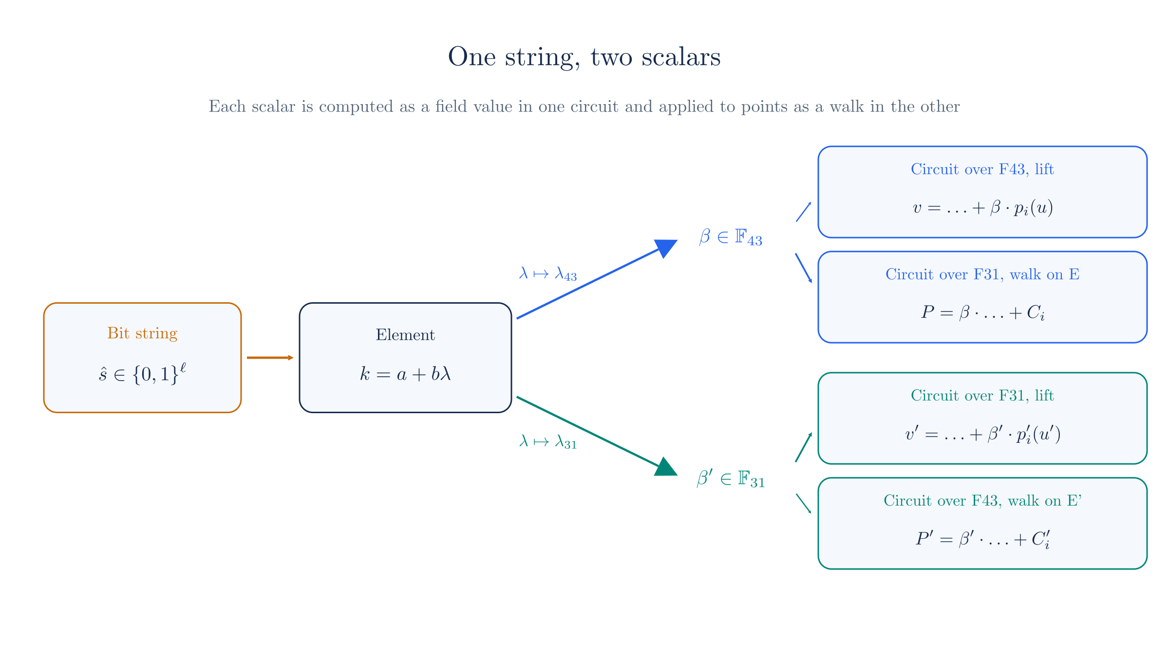
The bits are all that the two circuits share, and a bit is 0 or 1 in any field. Neither circuit ever handles a number from the other's field.

The same equality holds at full size. We ran it with Ragu's own test value:

The code's consistency test uses the endoscalar $206786806484900909362154774549736492353$. Our Python lift sends it to a scalar beginning 0x2d3c28380a8fb270... in ${\mathbb{F}}_q$ and a scalar beginning 0x26ea1541fb5a78a6... in ${\mathbb{F}}_p$. The walk on $(-1,2)$ on Pallas, in gates over ${\mathbb{F}}_p$, gives the same point as a direct multiplication by the first, and the walk on $(-1,2)$ on Vesta, in gates over ${\mathbb{F}}_q$, gives the same point as a direct multiplication by the second. Each walk took $480$ gates.

7. The walk in gates

Now we count, using the gates from the recursive proofs chapter, where a gate is one multiplication and a division counts as one multiplication checked backwards. A digit step has two parts, which are picking the digit's point and computing $3\cdot A+D$.

Tripling and adding

Done naively, $3\cdot A+D=((A+D)+A)+A$ is three additions at three gates each, or nine gates. Two of those gates compute $y$-coordinates of intermediate points that are never kept, so we try to remove them. Write $A=(x,y)$. The first addition has slope $t_1$, with $x_1=t_1^2-x-x_D$ and $y_1=t_1(x-x_1)-y$. The second addition has slope

$$t_2=\frac{y_1-y}{x_1-x}=\frac{t_1(x-x_1)-2y}{x_1-x}=-t_1-\frac{2y}{x_1-x}.$$

So $y_1$ has disappeared, and the slope equation becomes $(t_1+t_2)(x_1-x)=-2y$. The third addition follows in the same way, and only its output needs a $y$-coordinate. The code ends up with seven gates.

Picking the digit

Choosing among eight points would normally cost gates for each coordinate of each option, and the base point's coordinates are arbitrary wires. The code avoids this by first moving the point to a curve where its two coordinates are equal. The map $(x,y)\mapsto (c^{2}x,c^{3}y)$ takes $y^2=x^3+b$ to $y^2=x^3+c^{6}b$, for any nonzero $c$. Choosing $c=x/y$ makes both new coordinates equal to $r=x^3/y^2$, and the addition formulas never read $b$, so the walk can run on the new curve and move back at the end.

For $G_0=(1,2)$ on $E$, we get $c=1/2=16$ and $r=c^{2}x=8$. The new curve has constant $c^6\cdot 3=17$, and $(r,r)=(8,8)$ lies on it because $8^2=2$ and $8^3+17=2$ modulo 31.

On this curve the base point is $(r,r)$, so its free multiples are $(r,r)$, $(\zeta r,r)$ and $({\zeta }^{2}r,r)$. For the fourth digit we add $(r,r)$ and $-\varphi (r,r)=(\zeta r,-r)$. The slope is the constant $s=-2r/(\zeta r-r)=-2/(\zeta -1)$. From ${\zeta }^2+\zeta +1=0$ we get $(\zeta -1{)}^2=-3\zeta$ and $1/(\zeta -1)=({\zeta }^2-1)/3$, so the $x$-coordinate is

$$s^2-r-\zeta r=\frac{4}{-3\zeta }+{\zeta }^{2}r={\zeta }^2(r-\frac{4}{3}).$$

The $y$-coordinate is $s(r-x)-r$. Expanding with $s=-\frac{2}{3}({\zeta }^2-1)$ and using ${\zeta }^4=\zeta$ gives

$$y=-2{\zeta }^{2}r-r-\frac{8}{9}(\zeta -{\zeta }^2)=(1+2\zeta )(r-\frac{8}{9}),$$

where the last step uses $-2{\zeta }^2-1=1+2\zeta$ and $\zeta -{\zeta }^2=1+2\zeta$. All four digits therefore have coordinates that are affine in $r$:

Since each coordinate is $r$ times a constant, plus a constant, a selection needs only one product with $r$ per coordinate once the bits have been combined. Writing $p=e_1{e}_2$ and $q=ps$, we can read off an interpolation from the table:

$$\begin{array}{rl}{x}_D& =r(1+(\zeta -1)e_1+({\zeta }^2-1)e_2+(1-\zeta )p)-\frac{4}{3}{\zeta }^{2}p,\\ y_D& =r((1-2s)+2\zeta (p-2q))-\frac{8}{9}(1+2\zeta )(p-2q).\end{array}$$

For $e_1=e_2=1$ the first line gives ${\zeta }^{2}r-\frac{4}{3}{\zeta }^2$, and the second gives $(1-2s)(1+2\zeta )(r-\frac{8}{9})$, as the table requires. The products $p$ and $q$ would cost gates of their own. The plain gadget instead factors the selection so that it takes three gates in total, which we use here without deriving it:

We compared both selectors with direct point arithmetic for all eight digits at every affine point of both curves, which makes $576$ comparisons, and they all agreed.

One digit step

Here is the tripling on the normalized curve:

Here is the digit step for our string on $G_0$. The normalized accumulator is $A_0=(20,22)$ and the digit point is $D=(22,1)$.

So the result on the normalized curve is $(20,9)$, which three additions outside the circuit confirm. Dividing by $c^2=8$ and $c^3=4$ gives $(18,10)$, and that is $12\cdot G_0$. The tracer counted $20$ gates, namely 3 to normalize, 4 for the doubling, 10 for the digit and 3 to move back.

The start of the walk is cheap for a related reason. The tangent at $(r,r)$ has slope $3r^2/(2r)=3r/2$, which is linear in $r$. Then two gates compute the doubled point and two more apply the sign and the twist. With 47 digits, the total is $3+4+10\cdot 47+3$ gates.

Sharing the products

A fuse walks many points by one string, so each of those walks repeats the same products $e_1{e}_2$ and $e_1{e}_{2}s$. Ragu hoists them into a stage that the walk circuits share, and one circuit checks them once. Each digit then needs only the two products with $r$ from the equations above, which saves one gate per digit. Here are the costs together:

The last two rows come from running our tracer on the point $(-1,2)$ of Vesta with a 143-bit string, where it counted $480$ and $433$ gates and the result matched a direct multiplication by the lifted scalar. A circuit has $2^{11}=2,048$ gates, so it holds $1$ double-and-add multiplication or $4$ hoisted walks.

The hoisted count fits the limit of four endoscalings per circuit that Chapter 13 mentioned.

8. Why distinct strings stay distinct

Section 5 showed that strings name distinct elements of the ring, but the circuits work in the fields, and a nonzero ring element can have image zero there. Section 4 tells us when this can happen, so we bound the norm of a difference.

Take two strings and subtract their elements:

$$k-k^{\prime }=2\cdot 3^n(u-u^{\prime })+\sum _{i=0}^{n-1}{3}^{n-1-i}(d_i-d_i^{\prime }),$$

where $u$ and $u^{\prime }$ are the initial units. Units have absolute value 1, so $2|u-u^{\prime }|\le 4$, and digits have absolute value at most $\sqrt{3}$, so $|d_i-d_i^{\prime }|\le 2\sqrt{3}$. Weakening the 4 to $4\sqrt{3}$ gives a tidier result, and the geometric sum $\sum 3^{n-1-i}=(3^n-1)/2$ takes care of the rest:

$$|k-k^{\prime }|\le 4\sqrt{3}\cdot 3^n+2\sqrt{3}\cdot \frac{3^n-1}{2}=\sqrt{3}(5\cdot 3^n-1).$$

Squaring gives the book's bound on the norm, $N(k-k^{\prime })\le 3(5\cdot 3^n-1{)}^2$. The book states the bound without these steps, so the derivation is ours. If the bound is below the field size, the difference cannot have image zero, because of the divisibility rule in Section 4.

With 47 digits the bound is $3(5\cdot 3^{47}-1{)}^2$, which is about $2^{155.2}$, and the Pasta group orders are about $2^{254}$. A nonzero difference therefore cannot have a norm divisible by either order, and the 143-bit strings stay distinct in both fields.

The toy curves are far too small for this, and that makes them a useful illustration of what the bound prevents:

With one digit the bound is $3(5\cdot 3-1{)}^2=588$, and the largest norm that actually occurs among differences of our 32 strings is $228$. Both exceed 31 and 43, so the argument does not apply on the toy curves.

The 32 strings reach $21$ different scalars in ${\mathbb{F}}_{43}$ and $21$ in ${\mathbb{F}}_{31}$. For one clash, the strings 00000 and 11101 give the elements $7$ and $1-5\lambda$, whose difference $6+5\lambda$ has norm $31$, a multiple of 31. Both map to $7$ in ${\mathbb{F}}_{31}$.

There is also a second use of the norm. The walk uses incomplete additions, which divide by a difference of $x$-coordinates and so fail if the two inputs are equal or opposite. Let the accumulator have index $a$ and the digit have index $d$. The three additions need $a\ne \pm d$, then $2a+d\ne 0$ and $d\ne 0$, and then $3a+d\ne 0$ and $a+d\ne 0$. Each accumulator has absolute value at least 2 because of the initial doubling, and each later one is $|3a+d|\ge 3|a|-\sqrt{3}>|a|$, while digits have absolute value at most $\sqrt{3}$. So none of these combinations is zero in the ring. Their norms are again below the Pasta group orders, so none has image zero, and the circuit does not need to check these denominators at all. The walk relies on this by using an unchecked bank. On the toy curves the argument does not apply, and we can watch it fail:

We ran all 32 strings on every affine point of both curves, which makes $2,304$ walks. Every walk that finished gave the point the lift predicts. On $E$, $4$ strings failed with equal $x$-coordinates in an addition, and on $E^{\prime }$, $6$ failed. One failure on $E^{\prime }$ is the string 00011, with $A_0=2\cdot T$ and digit $1-\lambda$. After the first addition the accumulator is $A_0+D$, and adding $A_0$ again would give the index $2\cdot 2+(1-\lambda )=5-\lambda$, the norm-31 element from Section 4, which is the identity on $E^{\prime }$.

The same reasoning needs a base point with nonzero coordinates, since normalization divides by $y$ and by powers of $c$. A curve of prime order larger than 3 has no point with $y=0$, which would have order 2, and none with $x=0$, which would have order 3.

9. Extracting bits from a challenge

A transcript produces a field element, and the circuit needs its bits. A field element does not always have a unique bit decomposition inside a circuit, because a circuit checks ${\sum }_i{2}^i{b}_i=v$ modulo the field size. If the bits have enough room to exceed the field size, a prover can choose between spellings:

In ${\mathbb{F}}_{43}$ a 6-bit string can name values up to 63, so $21$ field elements have two spellings, one of them the value plus 43. The element $5$ can be written as 101000 or as 000011, which is $48=5+43$. These spellings have different low bits, 10100 and 00001, so they would name two different endoscalars. If we require the top bit to be 0, each of the 32 elements below $2^5$ has one spelling, and the $11$ elements from 32 to 42 have none and are rejected.

Ragu therefore requires the value to fit below $2^{\mathtt{CAPACITY}}$, the largest power of 2 below the field size, and then takes the low 143 bits of the unique spelling. Extraction also gives the right distribution:

Both Pasta primes lie just above $2^{254}$, so the capacity is 254 bits. The rejected values make up about $2^{-128.9}$ of ${\mathbb{F}}_p$ and about $2^{-128.9}$ of ${\mathbb{F}}_q$, which is the figure of about $2^{-129}$ in the source. Each 143-bit string has exactly $2^{111}$ in-range values above it, so a uniform in-range value gives a uniform string.

An honest prover almost never meets a rejected value. The grinding that Chapter 03 mentioned deals with the rare case for pre_beta, the last challenge of the transcript and the one that becomes $\beta$. There the prover re-randomizes the eval commitment and squeezes again until the value is in range.

10. Folding with an endoscalar

Now we can rerun the fold of Chapter 13 with the real map. Before doing so, we should separate the challenges that act on foreign points from those that do not. In the fold on the first side, the values $\alpha$ and $u$ only enter the computation of $v$, which is native to the circuit that folds values. Only $\beta$ also scales commitments, so only $\beta$ has to be applied through a walk. The code matches this on the native side, where it uses $\alpha$ and $u$ as full field elements.

The nested accumulator needs challenges of its own in ${\mathbb{F}}_{31}$, and it gets them by lifting the low bits of each native challenge. The nested ${\alpha }^{\prime }$ has no numeric relation to the native $\alpha$, and it does not need one, since the two batch different polynomials. For $\beta$ both sides lift the same string.

We keep Chapter 13's claims, namely $p_0$, $p_1$ on $E$ and $p_0^{\prime }$, $p_1^{\prime }$ on $E^{\prime }$. Section 8 showed that some toy strings hit an exceptional addition, so we picked a pre_beta whose walks all finish. Pasta needs no such choice.

Let the transcript give $\alpha =11$, $u=13$ and pre_beta $=31$ in ${\mathbb{F}}_{43}$, all below 32. The circuit over ${\mathbb{F}}_{43}$ uses $\alpha$ and $u$ as they are, and it lifts pre_beta to $\beta =12$. The circuit over ${\mathbb{F}}_{31}$ uses only lifts of the same bit strings, which are ${\alpha }^{\prime }=6$, $u^{\prime }=20$ and ${\beta }^{\prime }=5$.

Each value follows from the formula of Chapter 13 with its own scalars. Each point follows the same Horner form, starting from the commitment to $f$, with a walk in place of the double-and-add:

The decider then works directly with the polynomials, and it confirms the table:

The decider commits to the combined polynomials $p=(0,6,21,40)$ and $p^{\prime }=(9,4,19,4)$, and gets $(26,8)$ on $E$ and $(12,12)$ on $E^{\prime }$. It evaluates them at $u=13$ and at $u^{\prime }=20$, and gets $3$ in ${\mathbb{F}}_{43}$ and $9$ in ${\mathbb{F}}_{31}$. All four numbers match the table, although neither circuit ever computed in the other's field.

Here is how the cost compares with Chapter 13:

Each point now takes $46$ gates, two walks of $20$ and two additions of $3$, where the 4-bit double-and-add of chapter 13 took $68$ gates for a shorter challenge. Each circuit also pays $5$ gates to show that the bits are bits and $3$ gates to lift them.

The field value has to be the lift, because the walk acts as the lift. The plain integer now gives the wrong answer:

Suppose the circuit over ${\mathbb{F}}_{43}$ used the integer $31$ as $\beta$ in its field arithmetic. The walk on $E$ does not act as $31$. It takes the commitment $F=(28,10)$ to $12\cdot F=(24,30)$, while $31\cdot F=(24,1)$. The value and the point would then describe different polynomials, and the decider would reject.

11. Transcript bridging

The book's name for sharing one transcript between the two circuits is transcript bridging. Chapter 13 explained why it is sound only with input consistency. We now have the tools to say how the lifted values reach the nested side and how that side is held to them.

The nested circuits see no transcript. They read every challenge from a stage of their own trace, committed without blinding on the curve whose coordinates are native to the primary circuit. So its commitment is a known combination of generators, $C_s={\sum }_i\mathrm{lift}({\mathrm{ch}}_i)\cdot G_i$.

The native circuit holds each ${\mathrm{ch}}_i$ in its own field, and it cannot compute the lift, which lies in the other field. But walking $G_i$ by the bits of ${\mathrm{ch}}_i$ acts as exactly that lift, by the consistency property of Section 6, and $G_i$ has coordinates in the native field. Section 9 of Chapter 13 did this check with plain integers, and here is the real version:

The stage holds $({\alpha }^{\prime },u^{\prime },{\beta }^{\prime })=(6,20,5)$ with no blinding, on the generators $(20,3),(21,18),(25,18)$ of $E^{\prime }$ from chapter 13, and its commitment is $C_s=(2,31)$. The circuit over ${\mathbb{F}}_{43}$ holds the three transcript values as wires in its own field, breaks each into bits, and walks each generator by those bits. The walks give $(32,40)$, $(13,22)$ and $(21,18)$, which add to $(2,31)$ in $66$ gates. That circuit never computed $6$, $20$ or $5$, because it has no wires modulo 31, and it still confirmed a commitment to exactly those values. If the prover puts any of the $30$ other values in the place of ${\beta }^{\prime }$, the stage commits to a different point and the comparison fails.

So the endoscaling walk has two uses in a fuse. It folds commitments, and it also certifies foreign field values. The code divides the second use by timing. Four bind_challenges circuits handle two challenges each and export their partial sum. The challenge pre_beta comes last in the transcript, after the stage holding those partial sums has been committed, so its term has to wait. The next step's bind_beta adds it and compares the sum with the stage commitment, and for the root proof the verifier rederives the stage itself.

One gap remains. Each walk reads the bits from a stage as well, and we have to tie those bits to pre_beta. On the native side this is direct, because bind_endoscalar extracts the bits from pre_beta again and compares them wire by wire. The nested side cannot do this, because it holds no pre_beta. It has only the lifted ${\beta }_n$. So its compute_v circuit lifts its own bits and requires the result to equal ${\beta }_n$. This check is only as strong as the lift is injective, as the toy curves show:

The string 00100 also lifts to $5$ in ${\mathbb{F}}_{31}$, so a prover could load it into the circuit over ${\mathbb{F}}_{31}$ and pass the comparison with ${\beta }^{\prime }$. In ${\mathbb{F}}_{43}$ that string lifts to $5$ and not $12$, so the walk on $E$ now acts as $5$ and produces $P=(16,21)$ in place of $(26,8)$. The false accumulator has a value computed with $\beta =12$ and a point computed with $5$.

Among the 32 toy strings, $16$ pairs agree in ${\mathbb{F}}_{31}$ and disagree in ${\mathbb{F}}_{43}$. On Pasta no such pair exists, by the norm bound of Section 8.

This is the reason the book cares about injectivity, beyond keeping the sample space large.

12. Why cheating fails

We go through what a cheater can try, in the order of the sections above.

A second spelling of the challenge. Section 9 showed that a value with two bit decompositions would let a prover pick its endoscalar after the hash. The range requirement leaves one spelling. The verifier rejects a proof whose challenge is out of range, and no in-circuit assignment exists for such a value.

Wrong lifts on the nested side. The stage is unblinded and its commitment is recomputed from the transcript's bits, as Section 11 showed. Any other value changes the point, under the discrete log relation assumption for the generators of that curve.

Other bits in a walk. The native side compares its bits directly with the transcript. The nested side compares a lift, and on Pasta only one string has that lift.

A lucky challenge. A short challenge has a smaller range, as Chapter 13 counted. The lift adds a condition, which is that distinct strings must not pile up on the same scalar:

Take a cheater whose error in $v$ is the polynomial $\beta -c$, as in chapter 13. It passes when the string lifts to $c$. With an injective lift, one string out of the 32 would pass. On the toy cycle the lift is not injective, and the cheater does best with $c=0$, which $4$ strings reach, for a chance of $4$ in 32. So a collision in the lift directly raises a cheater's chance.

On Pasta the lift is injective in both fields, so each root of a fixed nonzero polynomial is hit by at most one string out of $2^{143}$.

The book adds up the roots charged to each challenge for one fuse step, and gets $66,477$ over all nine challenges. We recomputed that sum and the resulting $2^{-126.98}$.

The book calls this a conditional accounting for one step and not a security theorem, and it lists what a full argument would still have to cover, including an adversary's repeated Fiat–Shamir trials. We do not go further than that here.

Using an endoscalar for a secret. All of the above concerns public challenges. For a secret, the structure of the expansion helps an attacker, which is why the book and the code restrict endoscalars to public values:

Suppose the secret string is 00111, and an attacker sees $T=11\cdot G_0=(14,22)$. The attacker tabulates the 8 possible digit points, tries the 4 possible values of the head $2\cdot 3\cdot u$, and looks up $T$ minus each head in the table. That is 12 operations against 32 for trying every string, and the search finds the string. The saving grows with the width, because the expansion splits at any digit into a head and a tail that add up. At 143 bits the same idea takes roughly $2^{71.5}$ work.

That is far below the roughly $2^{127}$ work of a generic discrete log search in a group of $2^{254}$ elements, so a blinding factor must not be an endoscalar. A public challenge faces a different event, in which a fresh value hits a root that was fixed beforehand, and a meet-in-the-middle search does not apply to that.

The argument rests on these assumptions, and it is informal. Discrete log has to be hard on both curves, and the transcript hash has to behave as a random oracle. Every commitment has to enter the transcript before the challenges that test it, which is the input consistency of Chapter 13. The base points have to lie on the curve, which the circuits enforce separately. Each check also depends on a later step, so the decider has to finish the work at the root.

13. Feedback between the walks

A circuit does at most four endoscalings, so a walk over many points spreads over several step circuits. These step circuits have traces, and those traces have commitments, and the other side then has to fold those commitments too. Adding circuits on one side therefore adds work on the other side, and we need to know whether this settles at a finite number. The book treats this as a convergence problem.

Let $M$ and $N$ be the base number of endoscalings on each curve, and let $k$ be the capacity of one circuit. The book's model says that each circuit adds one endoscaling on the other curve. The first round needs $M/k$ circuits on one side. They add $M/k$ endoscalings on the other side, or $M/k^2$ circuits there, which add $M/k^3$ circuits back on the first side, and so on. Collecting the terms on one curve gives two geometric series with ratio $1/k^2$:

$$M_{\text{total}}=\frac{M}{k}(1+\frac{1}{k^2}+\cdots )+\frac{N}{k^2}(1+\frac{1}{k^2}+\cdots ).$$

For $M=N$ the sum is $M/3$ against a first round of $M/4$, which is a factor of $1.33$. The book also gives $k=8$, where the factor is $1.14$.

The code's batch has a different count. Its point formula is $1+2(\text{rx}+4)+6$, because a fuse folds the commitments of both children, so one more step circuit adds two points to the other walk rather than one. The other side's formula has the same shape. We can run the feedback from zero, with 22 fixed rx polynomials on the native side and 13 on the nested side:

The iteration stops at $23$ native steps and $26$ nested steps, the values that the code pins. With no feedback the first round would have been enough, with $25$ steps in all, so the feedback multiplies the count by about $1.96$.

Each step now adds 2 points to a walk that does 4 per step, so the ratio per round is $2/4$ and not $1/4$. For equal base counts the series sums to $(M/4)/(1-1/2)=M/2$, a factor of $2$, which agrees with the count above.

So the process converges in either model, and the factor is a modest constant. Section 14 records the difference between the two factors.

14. Endoscalars in Ragu

All of this describes the Ragu revision at 3219e08. Tachyon, which has not activated on mainnet and whose design is still changing, pins a different Ragu revision.

15. Where this chapter leaves us

This chapter took the following steps:

1. On a curve $y^2=x^3+b$ with a cube root $\zeta$, the map $(x,y)\mapsto (\zeta x,y)$ respects addition, and on a curve of prime order it multiplies every point by one scalar $\lambda$ with ${\lambda }^2+\lambda +1=0$.
2. Each field of a cycle keeps one constant, which acts on the coordinates of its own curve and as the eigenvalue on the partner curve, and these choices have to line up.
3. Elements $a+b\lambda$ have one image in each scalar field, and an image can be zero only when the field size divides the norm $a^2-ab+b^2$.
4. A string of $2+3n$ bits reads as an element through a radix-3 walk, whose eight digits are the nonzero residues modulo 3, so the element determines the string.
5. The walk costs ten gates per three bits, or nine with shared products, which makes 143 bits about three times cheaper than plain double-and-add.
6. On Pasta the norm bound keeps strings distinct in both fields and rules out exceptional additions, and the toy curves show both failures.
7. Extraction takes the low bits of the unique spelling of an in-range value, and a prover grinds pre_beta to stay in range.
8. A circuit lifts a string to get a field value in its own field and walks the string to act on foreign points, so one string serves both circuits with no foreign arithmetic.
9. The primary circuit holds the nested side to the lifted values by walking generators, and the nested side ties its bits to ${\beta }_n$ through injectivity.
10. Step circuits feed work back to the other curve, and the count settles at 23 native steps and 26 nested steps.

Several of these mechanisms depended on stages, including the challenge stage, the walk stage and the bridge stages. The next chapter explains how a circuit commits to its trace in parts and how the partial commitments are checked.