Recursion in Ragu
Part four built the pieces one at a time. We have a way to fold revdot claims, a registry that makes wiring cheap to check, endoscalars that let challenges cross the curve cycle, and stages that let circuits share data. This chapter puts them together into the operation that Ragu actually runs, and then follows a finished proof out of the tree.
The first half describes one fuse. We list what it has to do, the order of its messages, the circuits that divide the work, the split of the transcript between two of those circuits, and the public inputs they share. The second half describes compression, with a complete run on the toy curve, and then covers what the verifier pays, the size of the result, rerandomization, and the comparison with Orchard.
Reconstructed from code at commit 3219e08, not confirmed by the authors
The descriptions of the circuits and of compression follow the code and the book's recursion chapters. The numeric runs use small circuits of our own and a shortened instance, so they show the structure of the code and not its real contents. The sizes come from our reading of the code's wire format. We did not build or run the code, and we did not run its benchmarks.
Terminology
This site says fuse for the operation at a node of the tree, as chapter 02 explained, and native and nested for the two sides of the cycle, as chapter 13 explained. The decider is the check that runs when the recursion ends. The code writes pre_beta for the challenge from which is extracted.
1. What one fuse has to do
A fuse receives two child proofs and a step, and it has to produce a new proof that a parent can fuse in turn. Chapter 10 described the idea as a proof about a verifier. The children's verifier cannot run in full, so each child's expensive work joins an accumulator, and a fuse checks the cheap remainder inside its circuits. That remainder is still large, and a circuit may hold at most gates. These are the jobs:
| Job | Explained in | Where the code does it |
|---|---|---|
| Run the application's step | Chapter 02 | Application circuit |
| Replay the transcript to get the challenges | Chapter 03 | hashes_1, hashes_2 |
| Compute the children's from their public data | Chapter 10 | hashes_1, collapse |
| Fold the scalars of the revdot claims | Chapter 14 | collapse |
| Check the batched evaluation | Chapter 08 | compute_v |
| Connect the challenges to the other side of the cycle | Chapter 16 | bind_challenges, bind_beta |
| Fold the other curve's commitments | Chapter 16 | bind_endoscalar, endoscaling_step |
Dividing the jobs among circuits creates a new need, because the circuits have to agree with each other. They must use the same challenges, and they must read the same child data. Stages give them shared witness data, and Section 5 gives them shared public inputs. So a fuse produces many small traces where a textbook recursion step would produce one large one.
In the standard profile, one fuse therefore fills native polynomials, of which are circuit traces and are stages, and nested polynomials, and it adds the , , registry_xy and polynomials on each side, for in all. The native side folds revdot claims and the nested side folds .
Each internal circuit's claim counts once per child in the fold, since a parent checks both children's copies. All of these polynomials come from one call to fuse.
2. The order of the messages
Each challenge has to depend on everything it tests, so the order of the commitments is the backbone of a fuse. The code follows one schedule, and its phases sit in numbered files:
| Phase | File | What the prover computes | Challenge that follows |
|---|---|---|---|
| 1 | _01_application | The step's trace, with the headers | None |
| 2 | _02_preamble | A stage holding the children's data | |
| 3 | _03_s_prime | The restrictions for each child | , |
| 4 | _04_inner_error | and the first layer's quotients | |
| 5 | _05_outer_error | The second layer's quotient, the groups' values and the saved sponge state | |
| 6 | _06_ab | The new accumulator pair , | |
| 7 | _07_query | and the values that the registry claims | |
| 8 | _08_f | The batch quotient | |
| 9 | _09_eval | The value of every polynomial at | pre_beta |
| 10 | _10_p | The new batch polynomial and the walks over its points | None |
| 11 | _11_circuits | The traces of the internal circuits | None |
Nearly every row is a step of an earlier chapter. Phases 2 to 4 and 7 run the walk of chapter 15, phases 4 to 6 run the quotient fold of chapter 14, and phases 8 to 10 run the split accumulation of chapter 12.
Two details of the last rows matter later. Only pre_beta is ground, because it has to lie in the endoscalar range, so the prover re-blinds the eval stage and tries again until it does. And the internal circuits come last, because they prove statements about everything before them. Their traces feed no challenge of this fuse. Instead their commitments enter the parent's preamble, which puts them on the parent's transcript.
3. The internal circuits
We can now say what each circuit does. This table extends the one in Section 15 of the staging chapter, and it adds a column for the job:
| Circuit | Its job | Stages in its sum | Final mask |
|---|---|---|---|
hashes_1 | Derives , , , saves the sponge state, enforces the children's unified and that their circuit IDs are domain points | Preamble, outer error | Outer error |
hashes_2 | Resumes from the saved state and derives , , , , , pre_beta | Outer error | Outer error |
collapse | Enforces the children's application , and checks both layers of the fold down to | Preamble, inner error, outer error | Inner error |
compute_v | Computes from the query and eval stages, using the lift of | Preamble, query, eval | Eval |
bind_challenges (4 circuits) | Recomputes the nested challenge stage's commitment from the transcript's challenges | Preamble, query, eval | Eval |
bind_beta | Finishes that binding for each child, and ties the child's walked points to its unified instance | Points binding, preamble | Preamble |
bind_endoscalar | Ties the walk's bits to pre_beta, enforces curve membership, and exports the walk's end point | The five input points stages, walk | Walk |
endoscaling_step (23 circuits) | Performs 4 endoscalings of the Horner walk over the nested batch | The five input points stages, walk | Walk |
The stage column shows why stages were worth building. The hashes_1 circuit computes each child's and needs the child's data, which sits in the preamble. The collapse circuit reads that same data. Both read one polynomial, so a prover cannot show them different children, and only the bridge commitment has to enter the transcript.
The nested side has a shorter list. Its collapse checks the nested fold and pins its unified instance to the stages, its compute_v computes , and 26 endoscaling steps walk the native batch. The loading polynomial ties the walk's points to the bridge stages. That side has no transcript and no application circuit, as chapter 13 found.
The application's circuit uses no stages. All of the machinery above sits beside it and leaves its budget of gates to the application.
The stage chains
Book: the recursion chapter gives hashes_2 the chain preamble, outer error.
Code at 3219e08: hashes_2's claim sums only its own trace and the outer error stage, and its documentation marks the preamble as skipped. The layout still reserves the preamble's gates, which is what skipping a stage means.
This site follows the code.
4. Splitting the transcript
The transcript has to be replayed in circuit, because the Fiat–Shamir challenges would otherwise be numbers that the prover merely asserts. One circuit cannot hold the whole replay:
A permutation costs gates, and the code documents permutations in the first half and in the second. Together that makes permutations and gates, which already exceeds the limit of gates per circuit before any other check runs. The two halves cost and gates, so each fits.
So the replay has to cross a circuit boundary, and the sponge's state has to cross with it. The second circuit cannot recompute the state without repeating the permutations it is trying to avoid, and passing the state as a public input would add wires to every . The code places it in a stage. The state is known once the inner error bridge is absorbed, and the outer error stage is the next one committed, because it holds values folded with the that the state produces.
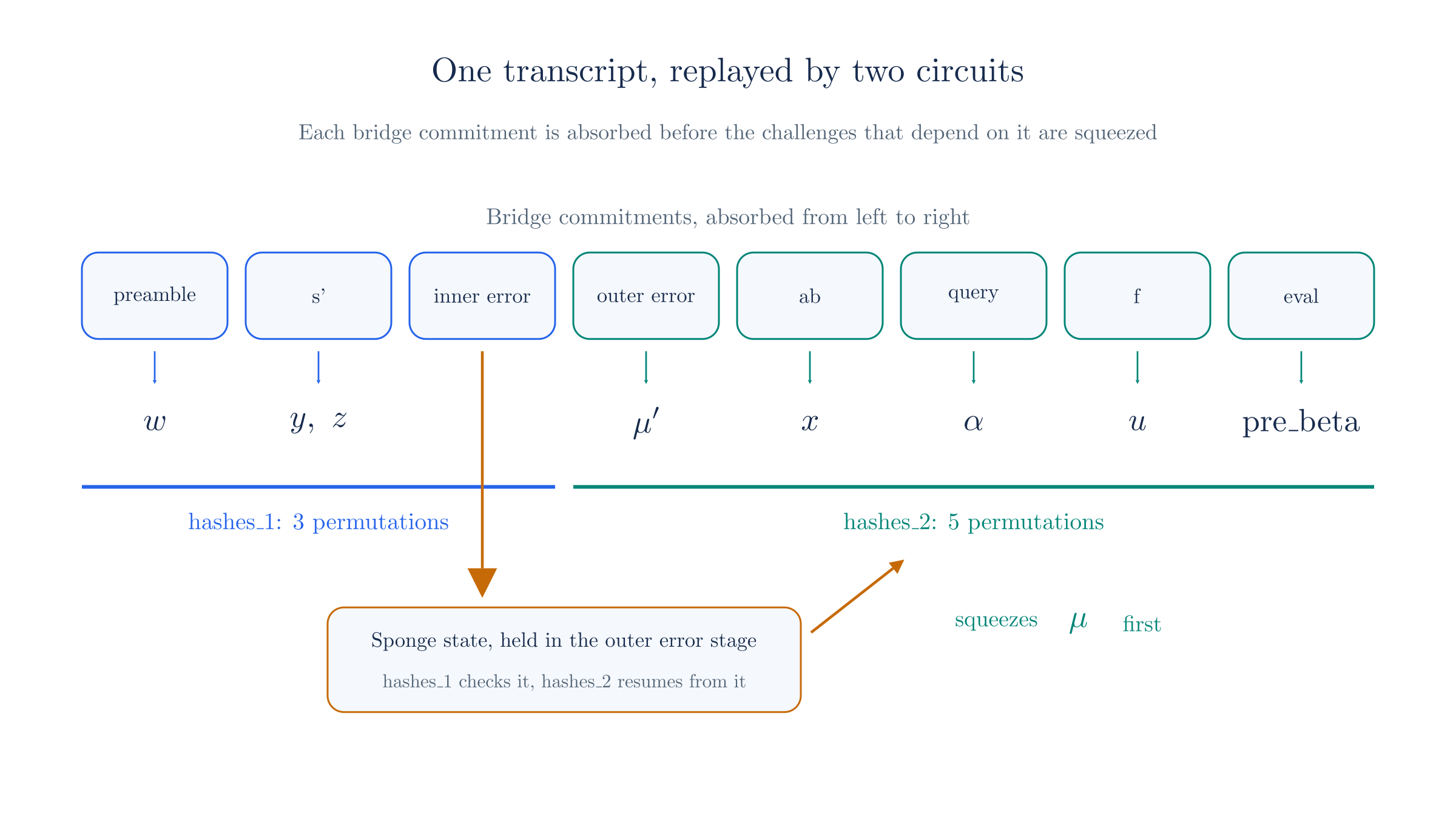
We run this on the toy sponge from chapter 03. The bridge commitments are points on , whose coordinates lie in , the field the sponge works in. The first point is the one chapter 17 built, and the others are stand-ins:
| Bridge commitment | Toy point on | Squeezed next | Replayed by |
|---|---|---|---|
preamble | hashes_1 | ||
s_prime | , | hashes_1 | |
inner_error | hashes_1, then saved | ||
outer_error | hashes_2 | ||
ab | hashes_2 | ||
query | hashes_2 | ||
f | hashes_2 | ||
eval | hashes_2 |
The first half ends by permuting and saving the three cells of the state, . The second half loads those cells and squeezes with no further permutation, which is why its count starts from the absorption of outer_error. We ran the sponge once straight through and once split at this point, and all nine challenges agree. The toy sponge takes permutations in the first half and in the second, as the code does, because we leave out the domain tag and its rate of 2 fits one point per permutation.
Reading the state from a stage leaves one question, which is what forces the stage to hold the right value. Only hashes_1 knows that value, having computed it, so the check goes in that circuit:
// save_state() applies a permutation (since there's pending absorbed data)
// and returns the raw state, ready for squeeze-mode resumption in hashes_2.
transcript
    .save_state(dr)
    .expect("save_state should succeed after absorbing")
    .enforce_equal(dr, &outer_error.sponge_state)?;
Without this line, a prover could pick the state and with it the challenges:
Suppose a prover wants , and it writes the state into outer_error. The second half alone would resume from this state and produce and . Of the possible states, give the wanted , but the first half compares the stage with the state it computed, and exactly state passes that comparison, the honest one. Both circuits read one committed stage polynomial, so the prover cannot show them different values.
5. Public inputs
Each circuit also has a public input polynomial , and a parent has to compute for each of a child's circuits. If every internal circuit exposed its own values, a parent would compute many different polynomials. The code avoids that with a unified instance, one structure of values that nearly all internal circuits expose in full, so that one computed serves them all.
Sharing an instance raises the question of who checks each value, since a circuit that merely exposes a value proves nothing about it. The code assigns each slot to exactly one circuit, and the prover asserts that all were covered. Other circuits read a slot as a witness, and the shared forces them to agree with the owner:
| Slots | Wires | Owner |
|---|---|---|
| Bridge commitments for preamble, and inner error; , , | hashes_1 | |
Bridge commitments for outer error, , query, and eval; , , , , , pre_beta | hashes_2 | |
collapse | ||
compute_v | ||
| The nested challenge stage's partial commitment | The last bind_challenges | |
| , , and the nested registry restriction | bind_endoscalar |
The rows add to points and elements, which is the code's wires.
Recursion uses three forms of over these values, plus a fourth with no wires of its own. All are Horner evaluations ending in the constant wire's 1:
Here Horner over wires and the final 1 means , so the last wire before the 1 is the coefficient of . The hashes_1 circuit uses , because it exposes the child headers, and the application circuit exposes the same headers through . Together those two claims stop a proof from using one pair of headers in the step and another in the recursion. An endoscaling step exposes nothing but the zero, so its polynomial is .
Take a toy unified output of five wires, , which are the first bridge point and the challenges , and from the run above. Take child headers and , whose second entry is the suffix, and the output header . At :
| Polynomial | Wires, in order | Value at | Coefficient of |
|---|---|---|---|
| Unified output, | |||
| Unified output, left, right, | |||
| Left, right, output | |||
| Endoscaling step |
Horner's rule reaches after the five unified wires, and both and continue from that value. Each table entry also matches a direct evaluation of the polynomial.
These values reach the fold through the parent. Its hashes_1 and collapse circuits compute each child's values from the preamble stage with gates, at the of the current fuse, and those values become the targets of the claims being folded.
The unified instance
Book: the public inputs chapter says that the shared structure holds 29 wires, from eight commitments and thirteen field elements. The recursion chapter's list gives nine challenges and two final values, which makes eleven elements. The public inputs chapter also says that four internal circuits share .
Code at 3219e08: thirteen points and eleven elements, which makes the 37 wires above. The five additional points are in the last two rows of the table. The count of circuits sharing is nine, because bind_challenges has four instances.
This site follows the code.
6. Keeping internal and application circuits apart
The registry holds internal and application circuits side by side, and a proof names its application circuit by a domain point the prover selects. So a prover could try to name an internal circuit and claim its trace as an application step. To rule that out, the code makes the two kinds of unable to coincide. Each internal circuit ends its output with a zero, and each application header ends with a suffix that is never zero.
Let an internal circuit expose wires and its zero suffix, so that , and let an application circuit expose a header , so that . If an application could use the suffix , then of the triples would make the two polynomials identical, and the swap would pass at every . For the difference depends only on and , so we tried all pairs of those, and none makes the polynomials identical. The two values then agree at no more than of the nonzero values of , and on a real field the same count is a negligible fraction.
This also explains why an endoscaling step needs the zero although it exposes nothing. Its comments say that the suffix is what stops a step from satisfying an application instance, given that the application's circuit ID may name any native slot. The nested registry holds internal circuits only, so it omits the zero.
The first application suffix
Book: application-defined suffixes begin at two, with one reserved for the trivial header.
Code at 3219e08: three values are reserved, with 0 for fixed circuits, 1 for the unit header and 2 for the Dummy header of the base case, so application suffixes begin at three.
This site follows the code. The book's argument is unaffected, since it needs only that the suffix is nonzero.
The value 2 has a job of its own, which chapter 10 described. Only the internal Bootstrap step declares the Dummy input, and only then does collapse waive its final comparison. The Rerandomize step has a witnessed suffix, so it constrains that wire away from 2.
7. What a proof carries to its parent
A parent does not repeat the checks in a child's circuits. It folds the child's claims into its own accumulators and reads the child's public data. Here is what it takes from a child:
| From the child | What the parent does with it | Explained in |
|---|---|---|
| Headers and unified instance | Holds them in the preamble and computes the child's values | Section 5 |
| Adds the pair as a raw claim with target , folded into the new | Chapter 14 | |
| Each trace and stage commitment | Adds a circuit claim or mask claim to the same fold | Chapter 17 |
| Adds the claim to its batch, folded into the new | Chapter 12 | |
| Opens it at the new , and opens its own new at the child's circuit ID, so one restriction remains | Chapter 15 | |
| Nested points and challenge partial | Walks the points and completes the challenge binding in bind_beta | Chapter 16 |
Three accumulators therefore pass up the tree, namely , and , one of each per side of the cycle. Each fuse replaces two of each with one, so a proof has the same shape at every depth. A child's internal circuits do not run again in the parent, and they cannot be skipped either, since their claims are among those folded.
The application's circuit sits in the registry like any other, and the base case runs through a single bootstrap proof. Chapter 10 records that the code has no Merkle root of initial states.
8. From a large proof to a short one
The accumulators stay few, but each one still holds polynomials of coefficients, and so does each stage and trace. A parent needs those polynomials to compute its fold. A verifier outside the tree does not want to receive them. The code's verify_uncompressed does hold every polynomial and checks the claims directly, and the code keeps it as a test oracle.
Compression replaces each polynomial with its commitment and a few of its values, and it restates the decider's checks so that those are enough. Chapter 09 ran this idea on one circuit. The book's compression chapter and the code arrange it in three reductions, which run once per curve:
The sections below run all three on the toy curve. We use the two circuits from the staging chapter, with and the sixteen generators listed there. We choose the challenges by hand. In the code a transcript under its own tag supplies them, after absorbing the instance and the output header, with fresh , , and on each curve.
9. The instance and its claims
The instance has to tell the verifier everything it would otherwise read off the polynomials. For our two circuits that gives this:
| Instance entry | Toy value | Role |
|---|---|---|
| , | , | Two stages. holds the values read from the registry |
| , | , | Final traces of the squaring and cubing circuits |
| , | , | The accumulator pair |
| Its stored revdot value | ||
| The restriction | ||
| , | , | The batch claim at the fuse's |
| , | , | The accumulator pair at that |
These numbers carry over from earlier chapters. The accumulator pair stands in for what the last fuse left, and we took the squaring claim at for it. The polynomial behind is chapter 06's example, with its opening point . The real instance holds a commitment for each native and nested polynomial, which makes it the largest part of the proof.
The verifier now rebuilds the decider's revdot claims from what it holds, in the order of the code's claim list:
| Slot | Claim | Kind | Left vector | Right vector | Target |
|---|---|---|---|---|---|
| 0 | Accumulator | Raw | |||
| 1 | Squaring circuit | Circuit | |||
| 2 | Cubing circuit | Circuit | |||
| 3 | Stage mask | Bonding | Mask of gate 1 | ||
| 4 | Final mask | Bonding | Mask of gates 2, 3 | ||
| 5 | Wire binding | Masked |
The first five claims have appeared in earlier chapters. The sixth exists because the decider also compares individual wires of certain stages against values it computes for itself, and a verifier that holds only a stage's commitment needs another way to make that comparison. The code turns it into a revdot claim. For wires at degrees with expected values , it sets
and the revdot product picks out the differences at those wires:
The target is 0, and it holds at a random only if each wire holds its expected value. The real list has five such claims natively and three on the nested side. In our run a small stage plays the role of the query stage:
The registry here has two circuits at and , whose wiring gives and . The stage claims those values in the wires and . With , the mask has a opposite and a opposite , and holds the expected values at those two degrees. So the product is . If the stage holds a wrong , the product is nonzero at all 43 values of . If both wires are wrong, the two errors cancel at one value of out of 43.
A real compressed proof has native claims, namely one accumulator pair, one application circuit, internal circuits, masks and wire bindings, and it has nested claims. In groups of , the native side has groups, first-layer terms and second-layer terms, and the nested side has groups, first-layer terms and second-layer terms.
10. Folding to three claims
Now the fold, in the form the code's compression uses. Chapter 14 noted that this differs from the fuse's quotient fold, and that the sources do not say why. Claim in group and slot takes the weights
and the folded pair is and . To see the target, expand the revdot product and separate the terms with :
The first sum holds the true targets . The other two terms collect the products that the verifier cannot compute, with for pairs inside a group and for pairs across groups. The verifier does not need those products individually. The prover lays them out as low coefficients of a vector for each layer, and the weights go in mirrored positions of a public vector , so that each is itself a revdot product, as chapter 14 showed. Our six claims fall into two groups of three, where the code uses seven per group:
With , , and :
| Value | Toy result |
|---|---|
| First-layer terms, group by group | |
| , committed before and | |
| Second-layer terms | |
| , committed before and | |
| , the target of | |
| , for comparison |
The vectors and have public parts that nobody needs to commit to, so the verifier separates what it derives from commitments and what it evaluates alone. A circuit claim's contains , so the committed polynomial takes care of that part at the dilated point :
Here holds the wiring restrictions, the terms, the masks and , and holds the expected values of the wire bindings. The commitments come from the instance:
The verifier obtains , and from small MSMs over the instance's points. Committing to the three polynomials directly gives the same points.
11. The split
We have three revdot claims, , and , and nothing has yet shown that any of them is true. The split from chapter 05 handles this. The prover combines the products with a challenge ,
and writes the result as . A revdot product is the coefficient of in the ordinary product, so that coefficient of is the combination of all three revdot products, and it lands in . This is the one place that pays for the product polynomial and its FFTs. The verifier then picks a point and checks the identity at it, and it sets aside its required value of to be opened later:
At the prover commits to and , and the required value is . At , so that and , it sends seven values:
The verifier adds what it can compute alone. It needs , and , the masks at , which are , and , and the two public vectors, and . That gives and , modulo 43. The left side of the split is , and the right side is .
The two sides agree, but all seven values are still only claims about commitments, which the next step settles.
12. Batching and the argument
The reduction leaves eight claims, seven from the values above and one for the required . The instance adds four of its own, which carry the fuse's accumulators into the check:
| Claim | Polynomial | Commitment | Point | Value |
|---|---|---|---|---|
| 0 | ||||
| 1 | ||||
| 2 | ||||
| 3 | ||||
| 4 | ||||
| 5 | ||||
| 6 | ||||
| 7 | ||||
| 8 | ||||
| 9 | ||||
| 10 | ||||
| 11 |
With only 43 points on the toy curve, some commitments repeat by chance, such as those of and . The polynomials themselves differ.
The last four rows are what the decider still owes from the recursion. Claim 9 is the fuse's accumulated , and claims 10 and 11 pin the values of the accumulator pair at that . Claim 8 is the restriction check of chapter 15:
Claim 8 opens at the fresh point . The verifier computes the value for itself, by evaluating the wiring of both circuits and combining the results with Lagrange weights, and this is the step that reads the whole registry.
Chapter 08's batch turns all twelve into one. The prover commits to the quotient and sends each polynomial's value at a new point . Then the verifier derives, with polynomials and claims,
Unlike the fuse's , which has to be short so that a circuit can scale points with it, this is an ordinary squeezed element, since no circuit runs this verifier.
With the quotient commits to . At the prover sends the eleven values . The verifier derives from those values and the claims. With this gives and , and the prover's polynomial agrees on both.
Now the inner product argument of chapter 07, in the code's form, proves :
The argument commits to the masking polynomial, , and takes and a multiplier on . The statement becomes . Then come rounds:
| Round | Challenge | ||
|---|---|---|---|
| 1 | 12 | ||
| 2 | 17 | ||
| 3 | 33 | ||
| 4 | 41 |
The final scalar is . The verifier computes from an MSM over all sixteen generators and from a product of four factors. The folded statement is , and , so the verifier accepts.
That finishes the run on this curve. In the code the same three reductions run again on the nested curve with its own claims, on one continuous transcript.
13. What the verifier pays
Chapter 09 named two linear costs, computing and computing , and part three set out to remove them from the circuits. They have not disappeared. No circuit pays them, which is what recursion needed, and the wiring chapter deferred the last piece to this page. The verifier of a compressed proof pays them once, at the root:
| Verifier step, per curve | Work | Growth |
|---|---|---|
| Replay the fuse transcript | permutations, on the native field only | Constant |
| Recompute two nested stages | Two small commitments, on the nested curve only | Constant |
| Compute targets | One Horner step per public wire | Size of the instance |
| Derive , , , | MSMs over the instance's points | Size of the instance |
| Compute for each circuit claim | native and nested circuits, one term per wiring coefficient | Linear in the circuits |
| Compute registry values for the wire bindings | One pass over the domain at , and natively further evaluations of | Linear in the registry |
| Compute | One pass over the registry, with Lagrange weights | Linear in the registry |
| Compute masks and | Closed forms | Logarithmic |
| Compute and combine the , | scalar multiplications and factors | Logarithmic |
| Compute | 1 MSM of scalar multiplications | Linear in the vector length |
The rows in bold are what remains of chapter 09's two costs. Wiring appears three times, because the compressed verifier evaluates each circuit claim's restriction at , the whole registry over its domain and at further points to fill the wire bindings, and the registry at the fresh . This last evaluation is the one chapter 15 described. It lets a whole tree of fuses rely on one restriction polynomial, since the verifier checks that polynomial against the full registry exactly once. Each of these passes grows with the wiring of the registered circuits, including the application's steps.
The last row is the deferred MSM of chapter 11. Compression computes it in full, with one per curve. None of these costs grows with the depth of the tree, so a proof that covers many leaves has the same verifier as a proof that covers two.
14. The size of the result
Counting from the code's wire format gives the following, for the standard profile at the production rank of 13 and headers of 4 elements, which is the size the code's benchmarks use:
| Part | Points | Scalars |
|---|---|---|
| Instance, commitments and values | ||
| Instance, two child headers of elements | ||
| Revdot reduction, per curve | ||
| Batch, per curve | ||
| IPA, per curve | ||
| Total, with two curves |
At 32 bytes per point or scalar, with 4 bytes for the circuit index and the 28-byte envelope, that comes to bytes. The uncompressed encoding writes coefficients for each of polynomials, which is bytes before counting its cached points, so compression shrinks the proof by a factor of about . Most of the compressed proof is the instance, with of its points. The IPA rounds, the only part that grows with the circuit size, take points.
The code's comment on profiles says "a few kilobytes", which agrees with this count.
A header larger than elements adds bytes per extra element, since the proof holds the two child headers. The output header does not count, because the verifier supplies it as the statement.
15. Why cheating fails
The chapters before this one each counted cheating at their own step. Here we look at what compression adds, which is the chance to hide a false claim in a value the verifier will never check directly. Start with a false public input:
Suppose the prover claims the output for the squaring circuit in place of , so its target rises by while its vectors stay honest. At our challenges the folded pair then misses by . Before the challenges, it can lower the term , whose weight is , by some amount . The false target adds to and the lowered term removes , so the fold balances only if . For that means , and we confirmed the balance there on the full vectors. Over all nonzero pairs , every nonzero balances exactly pairs, which is one value of out of 42.
The value is a second place to try:
After seeing and , the prover could raise alone and leave as committed. That can make balance, but it makes the claim false by the same amount, and arrives only after is fixed. We tried all nonzero shifts against all values of , and each shift passes at exactly value of .
The prover could also try to change the required value of directly:
Suppose the prover wants to be too large by . The coefficient of in is exactly , so whatever else it does, the difference from the true product is a nonzero polynomial of degree at most . The prover can choose the other coefficients of and to give that difference as many roots as possible, and we built such a pair. It passes the split at of the nonzero values of . This is the toy field's small size at work, since the same count on the real parameters is roots out of about values.
Once the split passes, every remaining claim is a statement about a commitment, and chapter 08 and chapter 07 already counted those. A prover cannot avoid the registry either, since the verifier computes both and each for itself. It cannot slip in a stray commitment, because every polynomial commitment the verifier reads gets opened through the IPA. The code's one exception is the nested challenge stage's partial commitment, which commits to no polynomial, and the bind_challenges claims hold it in place.
The argument above is informal, and it rests on these assumptions. Nobody knows a relation among the generators on either curve, so commitments bind. The two transcripts behave as random oracles, and each challenge comes after the commitments and values it tests. A false proof about a tree also has to get past the accumulation arguments of the earlier chapters. The book reports Lean proofs for some gadget contracts and says that these do not cover the protocol's overall soundness, which we do not establish here either.
16. Rerandomization and zero knowledge
A wallet would like two things from a proof beyond soundness. The proof should hide its witness, and when it reaches someone else it should not link back to the proof that produced it. As chapter 02 recorded, neither the Ragu Book nor the code at this commit establishes either property.
The code has an operation aimed at the second, rerandomize. It fuses the input proof as the left child with a cached proof of the unit header as the right child, under an internal step whose output header uses the same wires as the left input, so it cannot change the header. The result verifies as the input did. Both the book and the code say that unlinkability is the intention, and the comment on that function says that it is not achieved today. One of its reasons is that the fold is deterministic:
Reduce the fold to one commitment and let the output be , with the public weights and and the cached seeded point . An input of gives the output . An observer who wonders which proof went in can test each candidate against that equation. We tried all points as candidates, and only the true input matches.
The comment's other reason is more direct, because the output holds the input's commitments and stage polynomials in the clear as left-child data. It lists the remaining work as a randomizer in the fold and a way of hiding the child data.
Hiding the witness has a similar status. The stages' random is there to prevent cancellation and not for hiding, the IPA is unblinded at this commit, and the code says that a compressed proof is not hiding, because its openings are evaluations of the witness polynomials. To see what one evaluation can tell an observer:
Take the stage from chapter 17, where and one random entry sits at . Among all pairs , the commitment matches . Adding one value at a point, , leaves pairs, the true and also , because the commitment and the value together give a quadratic equation in . On a real curve nobody can list the commitment's matches, but the value still gives one linear equation in the secret wires, which is the sense in which the proof does not hide them.
This small case shows the effect of one value on one stage. A compressed proof opens combinations of polynomials at points the transcript chooses, so the leak there has a different shape, and we have not analyzed how much it reveals in practice. An uncompressed proof holds the polynomials themselves. The Tachyon book's description of stamps assumes zero knowledge, so this is an open requirement for Tachyon and not a settled property, as chapter 02 noted.
17. Performance against Orchard
The sizes above give a first comparison, which we can make from public formulas:
ZIP 225 gives an Orchard proof bytes for actions, which is bytes at and bytes at . So by our count a compressed Ragu proof with headers of elements is about the size of an Orchard proof for two actions, and one Ragu proof can stand for many transactions. The exact match at is a coincidence of these parameters.
For verification time, the book's analysis chapter gives a rough model, and it states that the figures need checking against benchmarks. It puts Orchard's batch verification at about 10 to 15 ms per proof on one thread, scaling as roughly . It estimates a Ragu proof at about 100 ms at , driven mainly by an MSM of points. Setting the two equal gives the crossover, with the cost per proof:
The book reports about 50 transactions with ms, and it does not state the base of the logarithm. We solved the equation at both ends of its range and for the two natural bases:
| Cost per proof in the model | ||
|---|---|---|
| ms | ||
| ms |
The book's figure sits inside the range the model allows, and the range is wide, as one would expect of a rough estimate. The shape of the curves is the more reliable conclusion. Batch verification of independent proofs keeps growing with the number of transactions, and verifying one aggregated proof does not.
The parameter gives a trade-off that the book leaves open. A larger circuit limit raises the verifier's cost for every proof and allows a shallower tree, and a smaller limit does the reverse.
The analysis chapter and the code
Book: the analysis chapter attributes the factor of 4 in to "the circuit structure across multiple stages", and it describes one MSM of points as the main cost.
Code at 3219e08: the number of coefficients is , and chapter 04 derives that factor from the four wires of each gate, independent of stages. A compressed verifier runs the checks on each curve, with one MSM per curve and the registry evaluations of Section 13. We read this as more work than the book's single MSM counts, which would raise the crossover, but we did not measure it.
The site follows the code for the structure and quotes the book for the estimates. The code has benchmarks for compression and compressed verification, and we did not run them, so we report no timings of our own. The book lists further analysis as future work.
These figures describe verification only. They leave out the prover's costs, which the sources do not quantify, and they compare with Orchard as it runs today, whereas Tachyon changes what a transaction carries. Tachyon has not activated on mainnet, its design is still changing, and it pins a different Ragu revision from the one this chapter reads.
18. Fusing after compression
One part of this design is still moving, and later chapters depend on it. Chapter 02 recorded that the Ragu Book calls a compressed proof terminal, while the code's profile comments foresee an Aggregator profile that verifies a compressed proof in circuit, with an internal Decompress step that outputs its header. The code says this has not landed, and a test pins the aggregator's shape to the standard one until it does. Such a circuit would have to run the verifier of Section 13 with gates, which is why the design places it in extra circuits that only aggregators carry. The chapter on aggregation returns to this.
19. Where this chapter leaves us
This chapter took the following steps:
- A fuse runs one transcript through eleven phases, each commitment coming before the challenge that tests it, and it divides the checks among many small circuits because each has at most gates.
- The replay takes more gates than one circuit holds, so
hashes_1andhashes_2share it, with the sponge state held in the outer error stage and checked by the first circuit. - The internal circuits expose one unified instance, with each slot owned by one circuit, so one serves them.
- Internal outputs end in zero and application headers end in a nonzero suffix, so the coefficient of keeps the two kinds of circuit apart.
- A parent folds three accumulators per side from each child, namely , and , so a proof keeps its shape at every depth.
- Compression replaces polynomials with commitments and values, through three reductions on each curve, from revdot claims to openings, from openings to one claim, and from that claim to an IPA.
- A wire binding turns the decider's comparisons of stage wires into revdot claims that a verifier can check from commitments.
- The compressed verifier pays the deferred linear costs once, as registry evaluations and one MSM per curve, and those costs do not depend on the tree.
- By our count a compressed proof takes bytes, against more than uncompressed. Rerandomization and hiding are not yet established, and the comparison with Orchard remains an estimate.
That completes Ragu as a proof system. The next part turns to what Tachyon proves with it, starting with notes, nullifiers, and tachygrams.