Staging
Up to now a circuit's trace has been one polynomial , committed all at once. The curve cycles chapter already had to break that habit, because a nested commitment only works if it covers part of a trace that some other circuit runs on. That chapter showed the idea on a short vector and promised the full mechanism here.
We split a trace into pieces that are committed separately, find out what can go wrong when the pieces are added back together, and build the check that prevents it. Then we use the pieces for the two jobs Ragu needs them for, which are sharing data between circuits and committing to data before a challenge. The chapter closes with a difference that chapter 13 left open, because the book adds the commitments of the pieces and we found no such addition in the code.
Reconstructed from code at commit 3219e08, not confirmed by the authors
The trace layout, the masks and their closed form below follow the code. The small circuits are our own, because the toy curves have too few points to serve as generators for one of Ragu's real circuits. The script behind this page runs each of them with the real gate and wiring equations.
Terminology
The book's staging chapter calls the pieces stage polynomials, or partial traces, and calls the remainder the final trace . The code's module documentation says staging polynomials and writes the remainder as , while builder.rs in the same directory writes . This site says stage polynomial and , because already means the combined quotient of chapter 08. We say primary and secondary for the two circuits of a cycle until Section 15, which uses the code's native and nested, as chapter 13 explained.
1. Two jobs for a partial commitment
Two situations in a recursive step call for committing to only part of a trace.
The first is a challenge in the middle of a circuit. Suppose a circuit holds many wires and would like to check something about them with a random linear combination. The challenge must depend on those wires, or the prover could pick the wires to suit the challenge. So the circuit has to hash them, and hashing inside a circuit is expensive. A commitment offers a cheaper route, since it binds all the wires under the same assumption as any Pedersen commitment and takes only two coordinates to hash:
The toy sponge from chapter 03 has rate 2, and one permutation applies S-boxes of multiplications each, or gates before counting anything else. Hashing wires takes permutations and gates. Hashing the two coordinates of a commitment to those same wires takes permutation and gates, and that cost stays the same however many wires the commitment covers.
The same trade appears in Ragu itself. The first transcript circuit absorbs three bridge commitments with three permutations, and the stages behind those commitments hold many more wires than the two coordinates of each point:
The native preamble stage reserves values for a header of elements, which is at least even for an empty header.
The second situation is data that several circuits have to read. The recursive proofs chapter noted that Ragu divides its verifier into many small circuits, and these circuits work on the same child proofs. Passing the shared data through public inputs would make every shared wire a term of that a verifier has to evaluate, and it would also publish any wire that is meant to stay secret. It would be better for each circuit to read the data as if it were part of its own witness.
Both jobs need the same thing, which is a commitment to some of the wires of a trace, made before the rest of the trace exists.
2. Splitting a trace
Commitments add, so a trace can be divided into parts that each get their own commitment. We write
where is a stage polynomial and is the final trace. With a second stage this becomes , and so on. The prover commits to and and does not need to commit to their sum, because the commitment to a sum is the sum of the commitments.
We need a small circuit to work with. Keep the secret from the arithmetization chapter, and start with the statement , which takes one multiplication. The trace uses the layout from Section 8 of that chapter, including the system gate at index 0 that chapter 09 introduced. We take gates, and we reserve gate 1 for the stage. The stage holds , and it also holds , which the next circuits will use.
A vector of entries needs 16 generators. We use the twelve from chapter 09, followed by . This chapter never uses the blinding generator , for a reason Section 3 gives.
Here are the two parts and their sum:
| Polynomial | Coefficients of | Commitment |
|---|---|---|
| Stage | ||
| Final trace | ||
| Sum |
Read gate by gate, with the stage's entry first and the final trace's entry second in each cell, the same numbers show which part supplies each wire:
| Gate | Reserved for | ||||
|---|---|---|---|---|---|
| 0 | System gate | 10 + 25 | 0 + 0 | 0 + 0 | 0 + 1 |
| 1 | Stage | 3 + 0 | 0 + 0 | 0 + 0 | 9 + 0 |
| 2 | Final trace | 0 + 3 | 0 + 3 | 0 + 9 | 0 + 0 |
| 3 | Final trace (unused) | 0 + 0 | 0 + 0 | 0 + 0 | 0 + 0 |
Gate 2 is the multiplication . Its copies of come from the wiring, with rows and , so the circuit's constraints reach across into the wires of the stage. That reach is the purpose of the arrangement, since the final trace never has to hold in the reserved slot.
3. Gates that hold free values
The consolidated equation from the arithmetization chapter applies to the sum , and it includes a gate check for every gate. A stage's gate has to pass that check for whatever values the stage holds, because the stage is committed before anything else is known about the circuit.
The wire allocator achieves this by writing each value to the wire of a new gate with , and it writes the next value to that gate's spare wire. So the gate has the form , which is why a stage carries two values per gate. The two gate equations from chapter 04 then read and , and they hold for any values:
We tried all pairs of values for , with . Every pair satisfies both equations of gate 1.
So a stage's gates do no checking of their own. They are storage, and any meaning the values have comes from constraints in the circuits that read them.
The system gate needs separate care. A real circuit has , but a stage has no such wire, so a stage that held only zeros would commit to the identity point, and a stage with predictable entries could cancel in a combination of commitments. The prover therefore places a random value at of each stage, which is the first number in the column of gate 0 above. This entry takes the place of in this chapter. It is not there for hiding, as chapter 09 recorded. The final trace has its own and supplies . Gate 0 passes because its and are zero.
With those two points settled, the consolidated equation applies to the sum as it does to any trace:
The right vector at and gives , and . The two sides agree at all pairs . The final trace alone fails at of those pairs, which shows that the circuit reads its input from the stage polynomial, not from .
4. Overlapping the stage
The split has a weakness. Adding polynomials adds their coefficients in every position, so nothing so far stops the final trace from putting a value in a slot reserved for the stage. To see what that buys a cheater, consider three equations:
Over , the equation has the single solution . The equation has the solutions , and they share . The equation has the solutions , neither of which solves the first equation.
Suppose a stage holds , which the cubing statement of chapter 04 needs, and a cheater wants to claim about that same stage. No single makes both true, but a stray entry can change what the second circuit reads:
Let the prover leave alone, so the stage still says , and put in slot of the final trace, whose gate 2 now holds . The sum then holds , and the circuit for accepts it at all challenge pairs, while the commitments still add up: . The commitment says one input and the circuit ran on another.
Chapter 13 saw the same effect on a shorter vector. A commitment check cannot find the problem, because a commitment to a sum equals the sum of the commitments however the entries overlap. We need a check that looks at where a polynomial's nonzero entries sit.
5. The stage mask
The requirement is linear in the polynomial's entries. A stage must be zero at every wire of every gate outside its reserved range, apart from the system gate. Let be that set of forbidden positions. Requiring many values to be zero is the task that a random combination handles, so we could ask for
at a random . If all the forbidden entries are zero, this holds for every . If any of them is nonzero, the left side is a nonzero polynomial in of degree at most , which has few roots.
This combination can be written as a revdot product, and that matters because revdot products are the claims that Ragu's accumulators fold. The revdot product pairs position with position , so we define a public vector with
Then
which is the combination we wanted. This is called the stage mask.
The mask is an ordinary wiring polynomial, for a circuit with an unusual shape. Take one constraint per forbidden wire, saying that the wire is zero. Section 11 of chapter 04 places each coefficient at the wire's partner position and weights row by . The code's test version of this circuit numbers the rows so that row is the constraint whose partner position is . The result is
Notice what is missing compared with the consolidated equation. A stage polynomial does not satisfy gates or the circuit's constraints on its own, so the claim has no dilation and no , and it has no public inputs, so its target is 0. The full claim is , in place of .
For stage , which reserves gate 1, the forbidden wires are those of gates 2 and 3:
| Gate | Wire | Position in the trace | Degree in the mask |
|---|---|---|---|
| 2 | 5 | 10 | |
| 2 | 10 | 5 | |
| 2 | 2 | 13 | |
| 2 | 13 | 2 | |
| 3 | 4 | 11 | |
| 3 | 11 | 4 | |
| 3 | 3 | 12 | |
| 3 | 12 | 3 |
At the mask for stage has coefficients . The stage has nonzero entries only at positions 6, 7 and 14, whose partners are 9, 8 and 1, and those are the positions where the mask has zeros. So the product is . The result is 0 at all 43 values of .
The final trace has its own mask, which forbids gate 1. Section 7 gives the details, but we can already apply it to the attack of the previous section:
The final trace from Section 4 has the stray entry at position 6, the partner of degree 9. Its product with the final mask is therefore , which equals at . It is zero only at , so 42 of the 43 values of catch it.
The cheater has more freedom than this, because the other three wires of gate 1 are also forbidden entries, and it can fill them in the hope of building roots. The product becomes , where , and are the entries it adds to , and . Trying all choices, the best one has nonzero roots, out of the 42 nonzero values of . Only of the choices also leave gate 1 satisfied, as the circuit needs, and the best of those has nonzero roots, at .
For the mask has degree at most in , so the bound is and the best rate we found is , counting . On a field of about elements with , the same bound falls below .
The book's description of the mask
Book: the staging chapter first says that wires outside the reserved range should be zero, and then says the mask enforces that everything must be nonzero inside the range.
Code at 3219e08: the mask forces wires to zero outside the range and says nothing about wires inside it.
This site follows the code, and it reads "nonzero" in the book as a slip for "zero outside".
6. A closed form for the mask
The verifier's two linear costs from chapter 09 included evaluating the wiring polynomial , since an arbitrary circuit has no structure to exploit. A mask does have structure, because it depends only on the product , and that makes it far cheaper. We derive the form the code uses.
Start from all degrees and remove the ones that are not forbidden. Let the stage reserve the gates starting at gate . The partner degrees of the wires of gate are for , for , for , and for .
For the system gate, gives the degrees , , and , whose powers of sum to
For the reserved gates, group the and wires, and then the and wires:
where the second line substitutes . Subtracting both groups from the full sum gives
The first two terms do not depend on the stage, and the code calls them the global mask. The last term is the notch for this stage. Each geometric sum has a closed form that takes multiplications, as in chapter 09.
Take and , so , and the mask of stage , for which and . The global term is and the notch is , so the formula gives . Adding over the eight forbidden degrees gives the same value. We checked the formula against the direct sum for every mask of this chapter at all 42 nonzero values of .
For a circuit with gates and a stage of gates, the mask has nonzero coefficients. The closed form needs only a few powers of and two geometric sums.
The registry computes the shared global term once, and each mask contributes only its notch. The chapter on wiring and the registry covers the registry itself.
7. A mask for every polynomial
Masks have to cover the final trace as well, because Section 4's attack put the stray entry there. The final trace has the same kind of mask, with the reserved range running from the end of the last stage to the top of the trace. In the code this is final_mask, and it uses the same type as a stage's mask with a larger count.
Stages also stack. A stage names its parent, and it starts where the parent ends, with a stage of values taking gates. Section 12 adds a second stage at gate 2, and with it our small circuits need these four masks:
| Polynomial | Gates it may use | Gates it must leave zero | ||
|---|---|---|---|---|
| 1 | 1 | 1 | 2, 3 | |
| 2 | 1 | 2 | 1, 3 | |
| Final trace after | 2 | 2 | 2, 3 | 1 |
| Final trace after | 3 | 1 | 3 | 1, 2 |
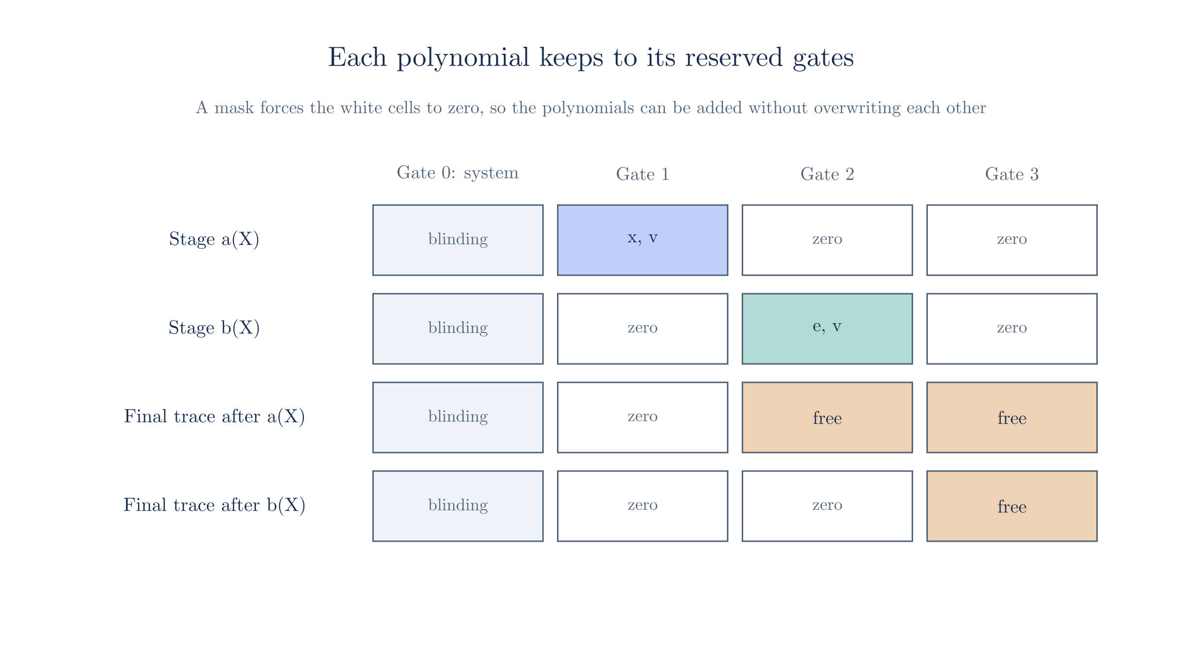
The system gate column is outside every mask, which is why each polynomial can have its own . The stage values fill only reserved gates, and the builder writes zeros in those slots of the final trace, so that the sum places each value in one spot.
A mask covers all four wires of its reserved gates, so a stage could in principle put values in its and . That gains nothing, because the gate equations on the sum still apply to that gate, and circuits read stage data only from the and wires.
8. Sharing one mask claim
A recursive step has two children, so it inherits the same stage twice, once from each. Each stage needs its mask claim checked. These claims can be combined, because the mask claim is linear in the polynomial:
The target stays 0, because mask claims have no public inputs that would need combining too.
Take the stage above as the left child's, and a right child's stage holding with . At the fold has coefficients , and its product with the mask is 0, as it is at all pairs . One claim did the work of two.
The folded claim still catches a bad stage:
Put a stray in gate 3 of the right stage. Among all pairs , the folded claim passes at , which are the 43 pairs with . Two stray entries at one position, one per child, can cancel each other at a single , since is a degree-1 polynomial in . Over all pairs of nonzero entries, no pair cancels at more than value of .
The same step does not work for a circuit's own claim, because appears twice in that equation. Substituting into the quadratic part gives
and the middle term has nothing to match it on the target side:
Fold two honest traces of the squaring circuit, with and with , in the same way at , and . The two claims are both true, but the folded product is while the folded target is . The terms with and do not match the target, and the two sides agree at only of the 43 values of .
Circuit claims therefore go through the error terms of the revdot folding chapter, and each one stays a separate entry going into that fold. Mask claims skip that cost, which the code's documentation lists as a property of gate-free claims.
The code also folds across circuits. Any polynomials with the same reserved range can share a mask, so the final traces of all the circuits that end on the same last stage fold into one claim. Section 15 shows this.
The order of the weights
Book: the combined claim is .
Code at 3219e08: the fold gives entry of the weight , so the first polynomial takes the highest power, as its module documentation also shows.
This site follows the code. The two orders are equally sound.
9. Two circuits on one stage
We can now do the second job from Section 1. Two circuits read the same stage by having the same polynomial inside their traces. The cubing circuit is the statement of chapter 04, with and read from the stage, and with one gate checking and another computing . Each circuit has its own final trace and its own wiring.
| Circuit | Statement | Trace | Commitment to its final trace | Consolidated equation |
|---|---|---|---|---|
| Squaring | Holds at all pairs | |||
| Cubing | Holds at all pairs |
The verifier holds three commitments and not four, because appears once and serves both traces. Neither statement mentions in its public inputs, and yet the shared commitment ties the two statements to one value. The difference shows when a prover tries the false pair of claims from Section 4:
With separate traces, the prover can use for the cubing circuit and for the circuit of , and each trace passes its own consolidated equation at every challenge pair. The verifier has no way to see that the inputs differ. With one shared stage the prover has to pick one , and the lists above show that no single value satisfies both equations.
Section 4's overlap was the only way around this, and the final mask closes it.
A circuit does not have to read every stage below its own. The builder can skip a stage, which keeps the layout the same but leaves those wires out of the circuit's constraints. The polynomial then does not join the circuit's sum at all.
10. Linking stages with a bonding polynomial
Sometimes the same value sits in two different stages, and the two copies need a check. In Section 12, stage carries a copy of that a circuit reads, and something has to tie it to the in stage . A circuit with one gate could do this, but the requirement is only a linear equation between wires, so it needs no gates at all.
The code provides for this case. A bonding polynomial is the wiring polynomial of a circuit that has only constraints, with no gates and an empty instance, and its claim has the same shape as a mask claim. A stage mask is the special case whose constraints each say that one wire is zero. The general case can compare stage wires with each other, and it is applied to the sum of the stages involved:
Such a polynomial is not allowed to reference the constant wire, so . That is why the row numbering below starts at 1.
The two stages hold in and . The only row of the polynomial is , placed at , because the position is empty in a polynomial of this kind. Then , which is 0 at all 43 values of . If stage holds in , the product at is , and only hides the difference.
Apart from the masks, Ragu's one such polynomial comes from the nested loading circuit, which requires each point used by the nested walk to equal the same point in the bridge stage that brought it in. Because the claim is linear, a grouped fold sums the stages within each child and combines the two children with .
11. What a mask does not check
A mask looks only at where entries sit, and it ignores their values. A stage whose wires are supposed to form a curve point or a bit passes its mask for any value:
A stage over that is supposed to hold a point of passes its mask for all pairs of coordinates, and only of those pairs lie on .
Constraints written while a stage is being built do not help, because the framework discards them. So some circuit that reads the stage has to state those constraints as its own. The code gives each reader a choice. Loading a stage enforced emits the checks in that circuit, and loading it unenforced relies on some other circuit to do so. Since the circuits read the same stage polynomial, one reader's check protects them all. For example, compute_v enforces the preamble while the other circuits load it unenforced, and bind_endoscalar enforces curve membership for the points stages.
12. Stages across the cycle
Now the first job from Section 1, a challenge that depends on the stage. Chapter 13 explained the difficulty. The commitment is a point on , so its coordinates lie in , and the sponge that derives challenges has wires in . The fix was a nested commitment, and we can now say exactly what that object is. It is a commitment to a stage of the circuit over , and the book calls this a nested staged commitment. Its stage holds foreign coordinates as ordinary wires, so it follows every rule above, including the layout, the and the mask.
| Step | Field | Result |
|---|---|---|
| Commit to stage on | scalars | |
| Place its coordinates in a stage of the other circuit, gate 1 | wires | , , with |
| Commit to that stage on | scalars | |
| Absorb the coordinates of and squeeze | wires |
In this way the challenge depends on and through two commitments, and the sponge absorbed only two wires. The circuit over reads the coordinates as its own witness, so it can run the deferred group operations on them:
The circuit over has gates, so it uses the twelve generators of from chapter 13. Its gate 2 is the first gate of adding to the fixed point . Holding , it checks modulo 31, with both differences written as linear rows over the stage wires. Its consolidated equation holds at all pairs , and both of its masks return 0 at all 31 values of . The toy curve has too few points for the two remaining gates of the addition, so we stop there.
The mask gives input consistency across the cycle in the same way as Section 5, so a prover cannot run this circuit on other coordinates than the ones the transcript absorbed:
Suppose the prover adds to slot in the final trace of this circuit, so that its gates run on the -coordinate while still holds . The final mask returns at , and only hides the entry. The same holds for all 30 nonzero amounts.
Back on the side, the challenge lets the prover commit to the next stage and finish the trace. Here we use to compress two wires of the stage into one value . Two wires make a small example, and the same reduction applies however many wires the stage holds:
With , the prover computes and commits to stage , which holds at gate 2, giving . The final trace holds one gate, , and . Rows of the wiring make and public, tie to , and require . The trace satisfies the consolidated equation at all pairs, with .
The combining circuit reads from stage , so it relies on the bonding polynomial of Section 10 to tie that copy to stage . The order of the commitments is what makes meaningful, as a target value shows:
Suppose the prover wants . With the stage fixed at , only one of the 43 values of gives that result, namely . If the prover could see before fixing the stage, it would set and reach the target for certain. Instead, every new changes , then , then . We ran that whole chain for the values of that give a usable commitment, and one of them, , reaches the target. A search of about 43 tries succeeds on a field of 43 elements, which is the repeated-trials problem from chapter 03, and the same search has no realistic chance on a 255-bit field.
The challenge itself reaches the secondary circuit by the route of chapter 13 and the endoscalars chapter. In the code, that route is one more stage, committed with , so that the primary circuit can recompute its commitment from the challenges.
Encoding the inputs on each side
Book: the PCS chapter gives two mirrored encodings, for the primary circuit and for the secondary, and treats them by symmetry. It places in the preamble stage as an advice wire and the rest of the tuple on public input wires.
Code at 3219e08: the design is not symmetric, because only the native side has a transcript. The native preamble and the points stages play the part of the book's , and their commitments go into bridge stages that play the part of . We found no separate absorbed on the nested side, which squeezes nothing. The roles of the wires are also reversed from the book's. The bridge commitment is a public value in the unified instance, and stage outputs stay private to the prover. The book's own public inputs chapter agrees with the code on that last point.
This site follows the code.
13. Adding the stage commitments
Chapter 13 recorded a difference that we can now settle. The book asks for two things about staged traces, that the parts do not overlap and that their commitments add up to the commitment to the overall trace. Sections 5 and 7 handled the first. In the book's form, the second looks like this:
In the circuit above, and the final trace commits to . The whole trace commits to . These are points on , so the next circuit over can add them with the gates of chapter 13, and the sum matches.
The purpose of this check is to tie the trace that the circuit's claim is about to the stage commitments that the transcript absorbed. A prover who committed to one and to unrelated stages would fail it.
The code reaches the same goal without a separate . A proof stores a commitment per stage and none for the whole trace, so there is no second object to compare. The circuit's claim is defined on the sum of its polynomials. Here is the line that lists the parts for compute_v, from crates/ragu_pcd/src/internal/native/claims.rs at commit 3219e08:
// compute_v: ComputeV + Preamble + Query + Eval
ComputeVCircuit => {
    for (((cv, pre), q), e) in source
        .rx(Rx(ComputeV))
        .zip(source.rx(Rx(Preamble)))
        .zip(source.rx(Rx(Query)))
        .zip(source.rx(Rx(Eval)))
    {
        processor.internal_circuit_claim(id, [cv, pre, q, e].into_iter());
    }
}
These claims then fold into one polynomial by the method of the revdot folding chapter. Two things follow. The prover can compute the commitment to with a small MSM over the stored commitments, and the verifying circuit recomputes the value of at a random point from the values of its parts. Each stored polynomial is opened at that point, and so is .
That gives the following run for our two circuits, with , and the opening point from and :
| Polynomial | Commitment | Value at the opening point | Weight in |
|---|---|---|---|
| 19 | |||
| 42 | |||
| 21 | |||
| 23 | Derived from the three rows above |
The prover gets the commitment to from three scalar multiplications, , and a commitment to the full polynomial gives the same point. The verifying circuit computes the expected value with field arithmetic and compares it with the opening of at that point.
A polynomial identity checked at a random point is enough, as in the encoding chapter, and the addition is linear, so it costs no gates. Evaluating at the shared point also means that a stage read by several circuits needs only one opening. A cheater who breaks the tie between stage and claim gets caught here:
Suppose the prover folds a squaring trace with stage input into , while the commitment in the proof still holds . The polynomial it commits to as then differs from the expected combination by a nonzero polynomial of degree . Of the 43 opening points, hide the difference.
Reconstructed from code at commit 3219e08, not confirmed by the authors
Book: the sum is checked in-circuit by the next circuit. The PCS chapter puts both kinds of check in the next secondary circuit.
Code at 3219e08: we found no such addition of points. The sum holds by definition of each claim, and the openings at tie the stored commitments to the folded claim. The stage checks are revdot claims on the native side and on the nested side, each folded by the parent with the rest of that side's claims.
This reading is ours, and the authors have not confirmed it. The site follows the code. The book's version remains a good way to understand the requirement, which is why this section and chapter 13 show it.
14. Why cheating fails
The sections above each counted one attack, so here we list what the protection rests on and add one more attack.
A prover can try to overlap the parts, and the stage and final masks catch that. It can try to give circuits different inputs, but they read the same stage polynomial, and the opening check ties the folded claim to the stored commitments. It can try to change a stage after seeing a challenge, but the commitment fixes the stage first, and through the bridge stage the commitment fixes the challenge. It can also try to supply a mask that suits its polynomial, but the mask for each stage is fixed in the registry, so it cannot select a different range. Checking against the wrong range fails in any case:
Check stage against the mask of , which forbids gate 1. The product is , or at , and it vanishes at only of the 43 values of .
The bonding polynomials also differ from circuit wiring in a way that blocks a substitution. Since for a bonding polynomial and for a circuit, a verifier that fixes for a circuit claim cannot be satisfied by a bonding polynomial in its place.
None of these claims is checked in the step that makes it. They join the accumulator, so a false stage leaves a false claim that the next step folds, and the decider rejects it at the end. The last step has no parent to do the checking, so the uncompressed verifier checks the root's own revdot claims, which include its mask claims with target 0.
The argument rests on these assumptions, and it is informal. Nobody knows a relation among the generators of either curve, so the commitments bind. The transcript hash behaves as a random oracle, each challenge comes after the commitments it depends on, and and come after the stage polynomials they test. A mask's check is only as strong as the degree over the field size, which is negligible for real parameters.
15. Staging in Ragu
The small circuits above match the structure of the real ones. The application's own circuit has a single trace with no stages, and the internal circuits are where staging happens.
Reconstructed from code at commit 3219e08, not confirmed by the authors
Native stages. They form a tree rooted at the points binding stage. One branch runs through the other points stages to the walk stage. The other runs to the preamble, which splits into outer error then inner error, and into query then eval.
Native circuits. Each circuit's claim sums its own trace with the stages it reads, and each final mask covers all the circuits ending on one stage.
| Circuit | Stages in its sum | Final mask |
|---|---|---|
hashes_1 | Preamble, outer error | Outer error |
hashes_2 | Outer error | Outer error |
collapse | Preamble, inner error, outer error | Inner error |
compute_v, bind_challenges | Preamble, query, eval | Eval |
bind_beta | Points binding, preamble | Preamble |
bind_endoscalar, endoscaling_step | The five input points stages, walk | Walk |
Nested stages. They form one chain, from the endoscalar and points stages through the bridge stages to the challenge stage. Each endoscaling step sums the first two. The nested collapse and compute_v circuits hold every stage. The loading polynomial of Section 10 covers the points stage and six of the bridges. The prover randomizes each ordinary stage's , as Section 3 required.
Mask claims. Every stage and final mask is one claim across both children, with no dilation and target 0. The saving is visible in the claim count:
In the standard profile, the native side has internal circuits, of which are endoscaling steps, along with stage masks and final masks. The count of revdot claims per fuse is . Each internal circuit counts once per child, and each mask counts once across both children, which saves claims.
The warnings in this chapter list where the book and the code differ. The chapter on recursion in Ragu walks through what these circuits compute. All of this applies to the Ragu revision at 3219e08. Tachyon, which has not activated on mainnet and whose design is still changing, pins a different Ragu revision and runs its steps against a mock of Ragu, so nothing at its pinned commit executes these stages.
16. Where this chapter leaves us
This chapter took the following steps:
- A trace can be split into stage polynomials and a final trace, each with its own commitment, so that some wires are fixed before the others exist.
- Stage values sit in gates of the form , which satisfy the gate equations for any values, so meaning comes only from circuits that read them.
- Adding parts can hide an overlap that no commitment check sees, so each part has a mask, which is a gate-free revdot claim that forbidden wires are zero.
- A mask depends only on , has a closed form, and folds across polynomials without error terms because its claim is linear with target 0.
- Circuits share data by including the same stage polynomial in their sums, and bonding polynomials compare wires between stages.
- A mask checks where values sit and not what they mean, so one reading circuit has to enforce the meaning.
- A nested staged commitment holds a commitment's coordinates in a stage of the other circuit, which lets the transcript absorb them and lets that circuit operate on them.
- The book adds stage commitments to reach a trace commitment. The code has no trace commitment, defines each claim on the sum of polynomials, and ties the result to the stored commitments by openings at a random point.
We now hold every part that the internal circuits use, namely folding, the registry, endoscalars and stages. The next chapter assembles them into the recursive step that Ragu runs.