Polynomial Commitments

The previous two chapters reduced a computation to claims about polynomials built from the prover's secret data. The verifier must now check those claims without receiving the polynomials. A polynomial with thousands of coefficients is too large to send in every recursive step, and sending it would also expose secret data. A polynomial commitment solves both problems by replacing the polynomial with one short value that the prover cannot later change.

This chapter builds the commitment Ragu uses. We start with a commitment to a vector, read a polynomial as its vector of coefficients, and then rewrite an evaluation $p(x)=y$ as a statement about an inner product. The next chapter proves that statement with a short argument.

1. What a polynomial commitment provides

Suppose a prover holds a polynomial $p$ and a verifier holds nothing. The two parties want to run the following exchange:

1. The prover sends a short commitment $C$ to $p$.
2. The verifier later picks a point $x$.
3. The prover sends $y=p(x)$ along with a proof that $y$ is correct for the polynomial behind $C$.

The verifier gets evidence about $p$ from one evaluation because two different low-degree polynomials rarely agree at a random point, as Statements and Challenges showed. This exchange only works if the prover fixes $p$ before seeing $x$, so the commitment must be binding: the prover must not be able to open $C$ to a second polynomial. When $p$ contains secrets, the commitment should also be hiding, which means $C$ reveals nothing about $p$.

A hash of the coefficients is binding and short, which makes it a natural first candidate. Hashes have no algebraic structure, however, so the only way to prove something about $p$ from its hash is to run the entire hash computation inside a proof. Ragu's accumulation scheme also needs to combine commitments directly, and the hash of a sum has no relation to the hashes of its parts. Elliptic curve points provide the missing structure, because adding two commitments gives a commitment to the sum. Sections 3 to 6 build this commitment and show why it has both properties. Sections 7 to 9 then connect it to polynomial evaluation.

2. The toy curve

The curve groups used in real systems have about $2^{255}$ elements, which makes their arithmetic unreadable on a page. Every worked example on this site uses a much smaller curve instead:

$$E:y^2=x^3+3\text{over }{\mathbb{F}}_{31}.$$

This curve has 43 points including the identity $\mathcal{O}$. The curves appendix lists the parameters.

Two different moduli

The worked examples use two different moduli, and it helps to separate them from the start. Coordinates of points belong to the field the curve is defined over, so we compute with them modulo 31. Here is one point operation carried out on coordinates:

Doubling $G_0=(1,2)$ uses the tangent slope, computed modulo 31: $s=3x^2/(2y)=3/4=24$. The new coordinates are $x_3=s^2-2x=16$ and $y_3=s(x-x_3)-y=10$, so $2\cdot G_0=(16,10)$.

Scalars count how many times we add a point to itself, and they behave differently. Adding a point to itself repeatedly eventually returns to $\mathcal{O}$, and the multiples then repeat:

One more addition gives $43\cdot G_0=\mathcal{O}$, and one after that gives $44\cdot G_0=G_0$. The multiples repeat with period 43, so only the value of a scalar modulo 43 affects the result.

The group has 43 elements, so scalars are computed modulo 43. Since 43 is prime, every point other than $\mathcal{O}$ generates the whole group in the same way. From here on, we write ${\mathbb{F}}_{43}$ for the scalars and treat point addition as a single operation.

Public parameters

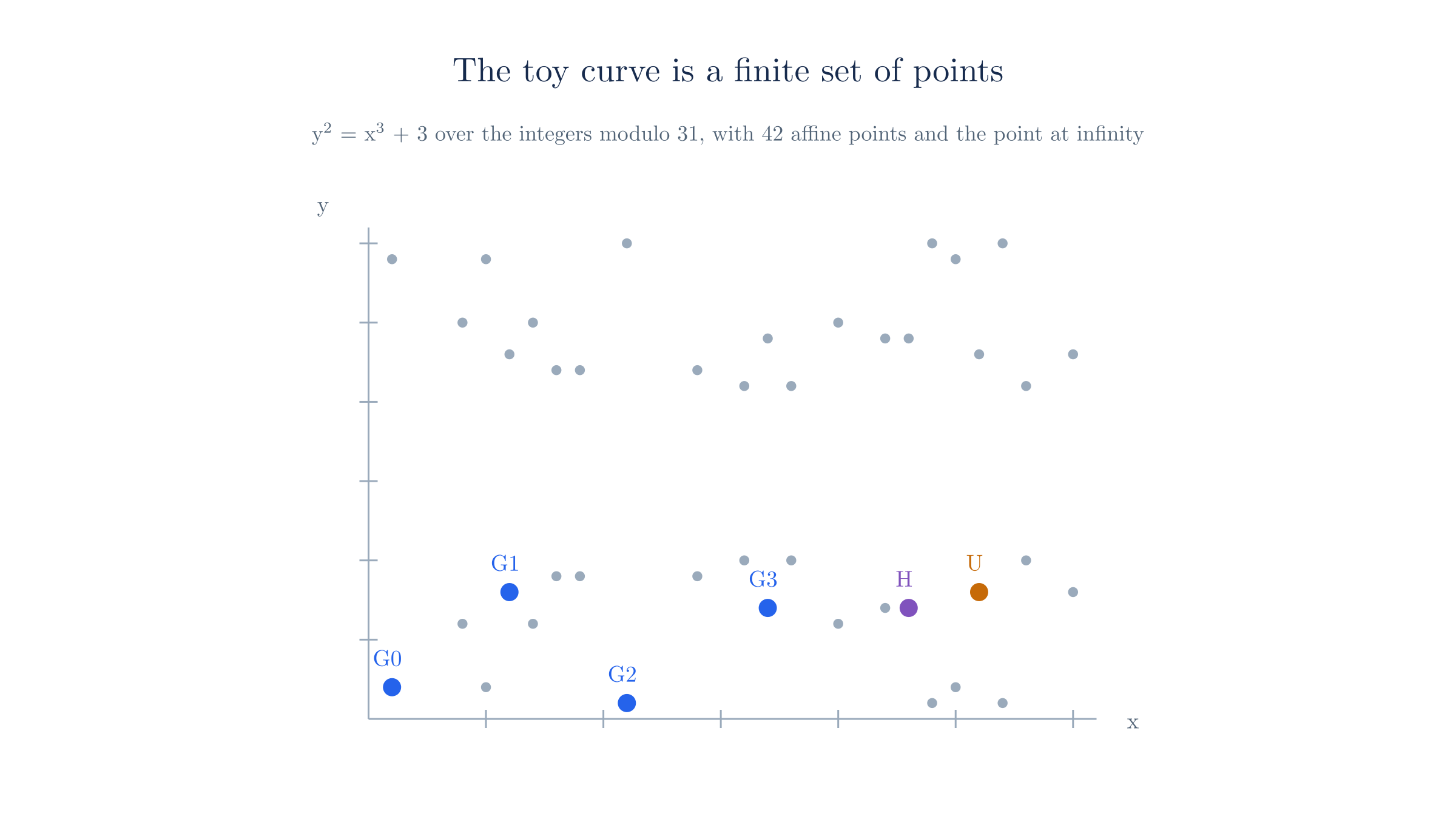
We fix six points as public parameters. A real system derives such points by hashing, so that no one knows a relation among them. The next table picks points spaced across the $x$-coordinates instead, which keeps the example readable.

The toy curve is deliberately insecure. Anyone can compute its discrete logs by counting, and Section 4 uses this weakness to show what goes wrong when a discrete log is known.

3. Committing to a vector

To commit to one scalar $a$, the prover could send $a\cdot G$ for a public generator $G$. This has both properties we want for a large group. Recovering $a$ from the point requires solving discrete log, which hides $a$ as long as it is hard to guess. The prover also cannot open the point to a second scalar, because the multiples of $G$ are all distinct until they repeat, so each point corresponds to exactly one scalar modulo the group order.

A vector needs more than this, since sending one point per entry would produce a commitment as long as the vector. Adding those points into one point keeps the size constant. If we used the same generator for every entry, the sum would be $({\sum }_i{a}_i)\cdot G$, which depends only on the sum of the entries and loses their positions.

The vectors $(7,2,5,3)$ and $(5,7,3,2)$ have the same entries in different positions. With $G_0$ in every position, both produce $17\cdot G_0=(20,6)$. With a separate generator for each position, they produce $(27,30)$ and $(26,8)$.

A separate generator for each position avoids this collision, because moving a value to a different position changes which generator multiplies it. For $\mathbf{a}\in {\mathbb{F}}_q^n$ and public generators $\mathbf{G}=(G_0,\dots ,G_{n-1})$, this gives the Pedersen vector commitment

$$C=⟨\mathbf{a},\mathbf{G}⟩=\sum _{i=0}^{n-1}{a}_i\cdot G_i.$$

The result is one curve point regardless of $n$. Here is the computation for a vector of four entries:

Take $\mathbf{a}=(7,2,5,3)$. Scalars live in ${\mathbb{F}}_{43}$, and each point sum follows the curve addition law over ${\mathbb{F}}_{31}$.

The commitment is the single point $C=(27,30)$.

4. Why a prover cannot change the vector

Suppose a prover opens the same commitment to two different vectors $\mathbf{a}$ and ${\mathbf{a}}^{\prime }$. Subtracting the two expressions for $C$ gives

$$\sum _{i=0}^{n-1}(a_i-a_i^{\prime })\cdot G_i=\mathcal{O},$$

where at least one coefficient is nonzero, since the vectors differ. A second opening therefore requires a nontrivial linear relation among the generators.

A relation of this kind is equivalent to knowing a discrete log. To see this for two generators, suppose $d_0\cdot G_0+d_1\cdot G_1=\mathcal{O}$ with $d_1\ne 0$. Moving the first term across and dividing by $d_1$ gives

$$G_1=-\frac{d_0}{d_1}\cdot G_0,$$

which expresses $G_1$ as a known multiple of $G_0$. If nobody can find such a multiple, nobody can open a commitment in two ways. Binding rests on this assumption, called the discrete log relation assumption. It also explains how real systems choose generators. If someone produced $G_1$ by multiplying $G_0$ by a chosen scalar, that person would know the relation and could forge openings, so real generators come from a hash whose output has no known relation to the other points.

On the toy curve we can compute such a relation directly, so we can run the argument above in reverse to produce a forgery:

Counting multiples of $G_0$ shows that $G_1=30\cdot G_0$, so $30\cdot G_0-G_1=\mathcal{O}$. Adding this relation to the honest vector gives ${\mathbf{a}}^{\prime }=(7+30,2-1,5,3)=(37,1,5,3)$ with scalars reduced modulo 43. Computing $⟨{\mathbf{a}}^{\prime },\mathbf{G}⟩$ gives $(27,30)$, the same point as $C$, so this commitment now has two valid openings.

The next table compares the two computations term by term. The change to entry 0 and the change to entry 1 cancel exactly, so the later terms and the total stay the same.

A prover who can do this on a real curve could change the committed polynomial after seeing the challenge. On a curve of 255 bits, no known method finds such a relation in practice.

5. Adding commitments

Point addition is commutative and scalar multiplication distributes over it, so we can regroup the terms of two commitments by generator:

$$\sum _i{a}_i\cdot G_i+\sum _i{b}_i\cdot G_i=\sum _i(a_i\cdot G_i+b_i\cdot G_i)=\sum _i(a_i+b_i)\cdot G_i.$$

Multiplying a commitment by a scalar $r$ regroups in the same way:

$$r\cdot \sum _i{a}_i\cdot G_i=\sum _i(r{a}_i)\cdot G_i.$$

Written with the inner product notation, these are two identities that hold for any vectors $\mathbf{a},\mathbf{b}$ and any scalar $r$:

$$⟨\mathbf{a},\mathbf{G}⟩+⟨\mathbf{b},\mathbf{G}⟩=⟨\mathbf{a}+\mathbf{b},\mathbf{G}⟩,r\cdot ⟨\mathbf{a},\mathbf{G}⟩=⟨r\mathbf{a},\mathbf{G}⟩.$$

Pedersen commitments are therefore linearly homomorphic, meaning anyone can compute a commitment to a linear combination of vectors from the commitments alone, without seeing the vectors. The toy curve confirms both identities:

With $\mathbf{b}=(3,1,8,4)$, the commitment is $C_b=(6,23)$. Adding points gives $C+C_b=(5,29)$. Committing directly to the sum $\mathbf{a}+\mathbf{b}=(10,3,13,7)$ gives $(5,29)$, the same point. Scaling works the same way: $6\cdot C=(11,30)$, and committing to $6\mathbf{a}=(42,12,30,18)$ gives $(11,30)$.

Much of the later construction depends on this property. Batched openings and accumulation both replace many committed polynomials with one random linear combination, and the verifier can compute the combined commitment using only group operations.

6. Hiding the vector

The commitment above is deterministic, so anyone who can guess $\mathbf{a}$ can recompute $C$ and test the guess. An observer holding $C$ can try one candidate after another:

This matters whenever the vector comes from a small set of likely values. Adding a term with a random blinding factor $\gamma$ and one more generator $H$ prevents this test:

$$\bar{C}=⟨\mathbf{a},\mathbf{G}⟩+\gamma \cdot H.$$

Hiding now follows from a counting argument. Fix any point $\bar{C}$ and any candidate vector $\mathbf{a}$. The difference $\bar{C}-⟨\mathbf{a},\mathbf{G}⟩$ is some group element, and because $H$ generates the group, exactly one $\gamma$ satisfies $\gamma \cdot H$ equal to that difference. Every candidate vector therefore explains the point equally well, so $\bar{C}$ alone gives no information about $\mathbf{a}$.

Committing to $\mathbf{a}$ with blinding factors $\gamma =17$ and $\gamma =29$ gives $(5,29)$ and $(18,21)$. Both differ from the unblinded $C=(27,30)$, and without the blinding factor an observer cannot test a guessed vector against either point.

The next example applies the counting argument to one specific point:

Take the blinded commitment $\bar{C}=(5,29)$ made from $\mathbf{a}$ with $\gamma =17$. The unrelated vector $\mathbf{b}=(3,1,8,4)$ also explains this point, using $\gamma =38$: $⟨\mathbf{b},\mathbf{G}⟩+38\cdot H=(5,29)$. An observer sees one point, and every candidate vector has exactly one blinding factor that fits it.

The other properties carry over. An opening now consists of the pair $(\mathbf{a},\gamma )$, and binding still holds under the same assumption once $H$ joins the list of generators, because two openings would again produce a relation among the points. Adding two blinded commitments gives a blinded commitment to the sum of the vectors, whose blinding factor is the sum of the two blinding factors.

7. Committing to a polynomial

A polynomial of degree less than $n$ is determined by its coefficients, which gives a direct route from vectors to polynomials:

$$p(X)=\sum _{i=0}^{n-1}{a}_i{X}^i⟷\mathbf{a}=(a_0,\dots ,a_{n-1}).$$

A commitment to $p$ is the Pedersen commitment to $\mathbf{a}$. Adding commitments now corresponds to adding polynomials, because adding polynomials adds their coefficients. The degree bound comes from the number of generators, so a set of $n$ generators can commit only to polynomials of degree below $n$. A polynomial of lower degree fits by treating its missing coefficients as zero:

The polynomial $6+X$ has degree 1, so its vector is padded with zeros to $(6,1,0,0)$. Its commitment is $6\cdot G_0+1\cdot G_1=(25,2)$, because the zero entries contribute $\mathcal{O}$.

The argument in the next chapter halves the vector in each round, which is why $n$ is a power of two.

8. Writing an evaluation as an inner product

Next we need a way to express $p(x)=y$ in terms of the committed vector. Expanding the definition of $p$ at a point $x$ gives

$$p(x)=\sum _{i=0}^{n-1}{a}_i{x}^i=⟨\mathbf{a},{\mathbf{x}}^{\mathbf{n}}⟩,\text{where }{\mathbf{x}}^{\mathbf{n}}=(1,x,x^2,\dots ,x^{n-1}).$$

An evaluation is therefore an inner product between the secret coefficient vector and a public vector, since anyone can compute the powers of $x$. The rewriting matters because the claim is now linear in $\mathbf{a}$. Each coefficient appears once, multiplied by a value the verifier already knows, and this is the same kind of expression as the commitment itself.

Let $p(X)=7+2X+5X^2+3X^3$ over ${\mathbb{F}}_{43}$, whose coefficient vector is the $\mathbf{a}$ from Section 3, and take $x=9$.

The last column sums to $y=37$ modulo 43. Direct substitution into $p$ gives $p(9)=37$, the same value.

Evaluations of linear combinations

Evaluation combines with the homomorphic property from Section 5. Evaluation is linear in the coefficients, so for any polynomials $p_a$ and $p_b$ with coefficient vectors $\mathbf{a}$ and $\mathbf{b}$, and any scalar $r$,

$$⟨\mathbf{a}+r\mathbf{b},{\mathbf{x}}^{\mathbf{n}}⟩=⟨\mathbf{a},{\mathbf{x}}^{\mathbf{n}}⟩+r⟨\mathbf{b},{\mathbf{x}}^{\mathbf{n}}⟩=p_a(x)+r{p}_b(x).$$

Commitments and evaluations therefore combine with the same coefficients. A verifier holding two commitments and two claimed evaluations can compute the commitment and the evaluation of the combination without seeing either polynomial.

Take $r=6$ with the vectors $\mathbf{a}$ and $\mathbf{b}$ from Section 5, each read as a polynomial, at $x=9$. Their evaluations are $37$ and $7$. The combined vector is $\mathbf{a}+6\mathbf{b}=(25,8,10,27)$, and its polynomial evaluates to $36$ at $x=9$, which equals $37+6\cdot 7$ modulo 43. Its commitment is $(7,6)$, which equals $C+6\cdot C_b$.

The chapter on batched openings uses this fact to reduce many evaluation claims to one.

9. Combining the commitment and the claim

The prover must now show two facts about one vector at once: $\mathbf{a}$ opens the commitment $C$, and $⟨\mathbf{a},{\mathbf{x}}^{\mathbf{n}}⟩=y$. Proving these facts separately would not be enough, since a prover could satisfy the first with one vector and the second with another. The two facts must apply to the same vector, so we package them into a single point. Taking the extra generator $U$, the prover and verifier both compute

$$P=C+y\cdot U,$$

and the prover claims to know $\mathbf{a}$ satisfying

$$P=⟨\mathbf{a},\mathbf{G}⟩+⟨\mathbf{a},{\mathbf{x}}^{\mathbf{n}}⟩\cdot U.$$

This form works because $P$ is a Pedersen commitment to the $n+1$ entries $(a_0,\dots ,a_{n-1},y)$ under the generators $(G_0,\dots ,G_{n-1},U)$. The binding argument from Section 4 now applies to the longer list. If the last entry is anything other than the true inner product, the prover must know a relation among these generators, including $U$.

To see why the same vector appears in both facts, read the two terms of the equation together. The vector that multiplies $\mathbf{G}$ is also the vector whose inner product with ${\mathbf{x}}^{\mathbf{n}}$ multiplies $U$, so one vector has to satisfy both parts. The verifier can compute $P$ from public values alone, because it holds $C$ and $y$.

The statement point is $P=C+37\cdot U=(5,29)$. Treating it as a five-entry commitment to $(7,2,5,3,37)$ under the generators $(G_0,G_1,G_2,G_3,U)$ gives $(5,29)$, the same point. A prover claiming $y=38$ instead has the statement point $C+38\cdot U=(1,29)$, which does not match the honest computation from the coefficients.

The generator $U$ must have no known relation to $\mathbf{G}$. If a prover knows those relations, the argument from Section 4 runs in reverse, as it did for the forged opening:

Counting gives the discrete logs of $G_1,G_2,G_3$ and $U$ relative to $G_0$: $30$, $28$, $25$ and $5$. The prover wants to claim the false value $y=38$, whose statement point is $C+38\cdot U=(1,29)$. With every point written as a multiple of $G_0$, the equation for $P$ becomes one linear equation over ${\mathbb{F}}_{43}$ in the four entries of the vector. Keeping entries 1 to 3 fixed and solving for entry 0 gives ${\mathbf{a}}^{\prime }=(15,2,5,3)$. This vector has inner product $2$ with the power vector, and $⟨{\mathbf{a}}^{\prime },\mathbf{G}⟩+2\cdot U=(1,29)$, so it satisfies the equation for the false statement point. The vector does not open $C$ and does not evaluate to $38$, yet the check passes.

Choosing the point after the commitment

The verifier also has to choose $x$ after the prover commits. If the order is reversed, one evaluation says little about the committed polynomial:

Suppose the prover learns $x=9$ before committing. It can then take $q(X)=p(X)+(X-9)=41+3X+5X^2+3X^3$, a different polynomial that has the same value at this point: $q(9)=p(9)=37$. A check at $x=9$ cannot distinguish the two polynomials, even though their commitments $(16,10)$ and $(27,30)$ differ.

When the commitment comes first, the prover has to fix the polynomial with no knowledge of $x$, so the random-point test from Statements and Challenges applies. A prover who commits to $q$ and hopes it matches a different polynomial $p$ at $x$, with both of degree at most $d$, has at most a $d/|{\mathbb{F}}_q|$ chance of success.

Take the different polynomial $q(X)=p(X)+2(X-1)(X-2)(X-3)=38+24X+36X^2+5X^3$. Evaluating $p$ and $q$ at all 43 points of ${\mathbb{F}}_{43}$ finds agreement only at $x\in \{1,2,3\}$. A uniformly random challenge therefore misses the difference with probability $3/43$, which is the Schwartz–Zippel bound for degree 3. On a curve the size of Pallas, the same bound is below $2^{-240}$ for any polynomial of the degree Ragu uses.

A complete run with the coefficients revealed

We can now run the whole exchange on the toy curve. In this version the prover finishes by revealing the coefficients, which gives the verifier everything it needs to check the equation directly:

This run confirms the claim, but steps 4 and 8 are the problem. Step 4 sends all $n$ coefficients, which exposes them and removes the size benefit of the commitment. Step 8 costs the verifier one group operation per generator. The next chapter replaces the reveal with a short argument:

For $n=2^{13}$ with 32-byte values, revealing the coefficients costs $8192\times 32=262,144$ bytes. An argument with $26$ group elements costs $832$ bytes, plus a small constant number of extra values.

We can now state exactly what that argument must prove:

$$\text{given }\mathbf{G},U,P,x,\text{ the prover knows }\mathbf{a}\text{ such that }P=⟨\mathbf{a},\mathbf{G}⟩+⟨\mathbf{a},{\mathbf{x}}^{\mathbf{n}}⟩\cdot U.$$

10. Comparison with KZG

The most widely known alternative is KZG, which takes a different route to the same interface. KZG requires a setup that publishes the points $G,\tau G,{\tau }^{2}G,\dots$ for a secret scalar $\tau$, and the commitment to $p$ is the point $p(\tau )\cdot G$. To open at $x$, the prover sends a commitment to the quotient $(p(X)-y)/(X-x)$, which is a polynomial exactly when $p(x)=y$. The verifier checks this relation at $\tau$ with a pairing, a special bilinear map between curve groups.

KZG proofs are one group element, and their verification cost does not depend on $n$. In exchange, KZG requires pairing-friendly curves and a trusted setup, because anyone who learns $\tau$ can forge openings. Ragu avoids a trusted setup and uses the Pasta curves, which Zcash already deploys in Orchard. The cost of that choice is a verifier whose work grows linearly with $n$, and most of the recursion chapters exist to manage this cost.

11. The commitment in Ragu

The core of Ragu's commitment function matches the definition from Section 3. The function asserts that the coefficient count is exactly $n=2^k$ and then runs a multi-scalar multiplication over the generators, here from crates/ragu_pcd/src/ipa/mod.rs at commit 3219e08:

pub fn commit<B: SelectableBackend>(&self, poly: &[C::Scalar]) -> C::Projective {
    assert_eq!(poly.len(), self.n as usize);
    msm::multiexp::<C, B>(poly, &self.g)
}

12. Where this chapter leaves us

This chapter took the following steps:

1. A Pedersen vector commitment compresses a vector into one curve point, with one generator per position.
2. Binding holds as long as nobody knows a relation among the generators, and a blinding factor adds hiding.
3. Commitments add in the same way as the vectors behind them.
4. A polynomial is committed through its coefficient vector, and its evaluation at $x$ is an inner product with the powers of $x$.
5. The point $P=C+y\cdot U$ combines the commitment and the claimed value into one statement about one vector.
6. A random $x$ chosen after the commitment makes one evaluation meaningful, because distinct low-degree polynomials rarely agree there.

Nothing yet makes the proof of the final statement short. The next chapter supplies that step by halving the vector repeatedly.